Taylor Dispersion Analysis: A Complete Guide for Precise Diffusion Coefficient Measurement in Biomedical Research

Abstract

This comprehensive guide explores Taylor Dispersion Analysis (TDA) for diffusion coefficient measurement, a critical parameter in biomolecular characterization and drug development. It begins with the foundational physics behind the method, explaining how hydrodynamic dispersion in a capillary relates to molecular diffusion. The article provides a detailed, step-by-step methodological workflow for experimental setup, data acquisition, and analysis using TDA. It addresses common experimental challenges and optimization strategies to ensure data accuracy and reproducibility. Finally, the guide validates TDA by comparing its performance, advantages, and limitations against established techniques like Dynamic Light Scattering (DLS) and Analytical Ultracentrifugation (AUC). Tailored for researchers and pharmaceutical scientists, this resource equips professionals with the knowledge to implement TDA for characterizing proteins, nanoparticles, and complex therapeutics.

What is Taylor Dispersion? Understanding the Core Principles for Diffusion Measurement

Within the broader thesis on the Taylor dispersion method for diffusion coefficient measurement research, this article details the evolution from Geoffrey Taylor's seminal 1953 publication to contemporary, automated laboratory implementations. The technique exploits the dispersion of a solute band in laminar flow within a capillary to extract precise diffusion coefficients (D), critical for understanding molecular size, interactions, and stability in drug development and material science.

Theoretical Principle & Evolution

Taylor's analysis showed that under conditions of laminar (Poisonille) flow, the axial dispersion of an injected solute plug is governed by a combination of convective flow and radial diffusion. The effective dispersion coefficient (K) is related to the molecular diffusion coefficient (D) by: K = (r²²) / (48D), where r is capillary radius and is average flow velocity. Modern adaptations use this relationship to calculate D from accurately measured dispersion profiles.

Table 1: Evolution of Key Parameters from Taylor's Setup to Modern Systems

Parameter	Taylor's Theoretical/Experimental Setup (c. 1953)	Modern Commercial Instrument (e.g., Flow-Induced Dispersion Analysis)
Capillary Dimension	Theoretical analysis; practical use of tubes of mm-scale radius.	Fused silica capillaries, typically 10-75 µm i.d., 50-100 cm length.
Flow Control	Pressure-driven or gravity-fed flow.	High-precision syringe pumps (nL/min to µL/min).
Detection Method	Offline sampling or refractive index.	On-line UV/Vis, fluorescence, or mass spectrometry detection.
Sample Volume	Not explicitly minimized (mL scale).	Nano- to micro-liter injections.
Data Analysis	Manual calculation from concentration profiles.	Automated software for peak fitting and D calculation.
Typical D Measurement Range	Analyzed for large-scale phenomena.	10⁻¹² to 10⁻⁹ m²/s, suitable for proteins, aggregates, nanoparticles.
Primary Application in Thesis Context	Foundation for dispersion theory.	High-throughput biomolecular interaction analysis, binding affinity, size distribution.

Detailed Experimental Protocols

Protocol 1: Basic Diffusion Coefficient Measurement via Taylor Dispersion

Objective: Determine the diffusion coefficient of a standard fluorescent dye (e.g., FITC) to validate system performance. Materials: See "Scientist's Toolkit" below. Procedure:

• System Preparation: Flush capillary sequentially with 1M NaOH (30 min), deionized water (30 min), and running buffer (e.g., 10 mM phosphate, pH 7.4) for 60 min using a high-pressure pump (~5 bar).
• Thermostating: Place the capillary coil in a thermostated cartridge or bath set to 25.0 ± 0.1 °C. Allow equilibration for 30 minutes.
• Sample Preparation: Prepare a 10 µM FITC solution in running buffer. Prepare a vial of running buffer for blank.
• Injection & Run: a. Set syringe pump to a precise, low flow rate (e.g., 50 nL/min). b. Using an injection valve or pressure, inject a 5 nL plug of the FITC sample into the capillary flow. c. Immediately switch flow to running buffer. Maintain isocratic flow. d. Start data acquisition from the on-line fluorescence detector (Ex: 494 nm, Em: 525 nm).
• Data Acquisition: Record the dispersed peak until it returns to baseline. Save the high-resolution temporal profile (C(t)).
• Data Analysis: a. Fit the resulting peak to the Taylor dispersion equation: ( C(t) = \frac{C0}{\sqrt{4πK t}} \exp\left[-\frac{(L/ - t)²}{4K t}\right] ), where L is capillary length. b. Extract the variance (σt²) of the peak. Calculate K = (σ_t² ³) / (2L). c. Calculate D using the rearranged Taylor equation: ( D = \frac{r²²}{48K} ).
• Validation: Compare obtained D value with literature (e.g., ~3.0 x 10⁻¹⁰ m²/s for FITC in aqueous buffer at 25°C).

Protocol 2: Binding Affinity Measurement (Kd) via Size-Shift Analysis

Objective: Determine the dissociation constant (Kd) for a protein-ligand interaction by monitoring the change in diffusion coefficient of a fluorescent ligand upon binding. Materials: Target protein, fluorescent ligand, assay buffer. Procedure:

• Ligand Alone Control: Perform Protocol 1 for the fluorescent ligand at a concentration << expected Kd. Record D_ligand.
• Titration Series: Prepare a series of samples with constant fluorescent ligand concentration (e.g., 50 nM) and varying target protein concentration (e.g., 0, 25, 50, 100, 200, 500 nM). Equilibrate for 30 min.
• Sample Analysis: Run each sample from step 2 using Protocol 1 steps 4-6. For each run, calculate the apparent diffusion coefficient (D_app).
• Data Processing: a. The change in diffusion coefficient (ΔD = Dapp - Dligand) is proportional to the fraction of bound ligand. b. Plot ΔD (or Dapp) versus the total protein concentration. c. Fit the data to a 1:1 binding isotherm: ( ΔD = ΔD{max} \frac{[P]total}{Kd + [P]total} ), where ΔDmax is the ΔD at full saturation. d. The fitting yields the Kd value.
• Quality Control: Include a non-binding control protein to verify specificity.

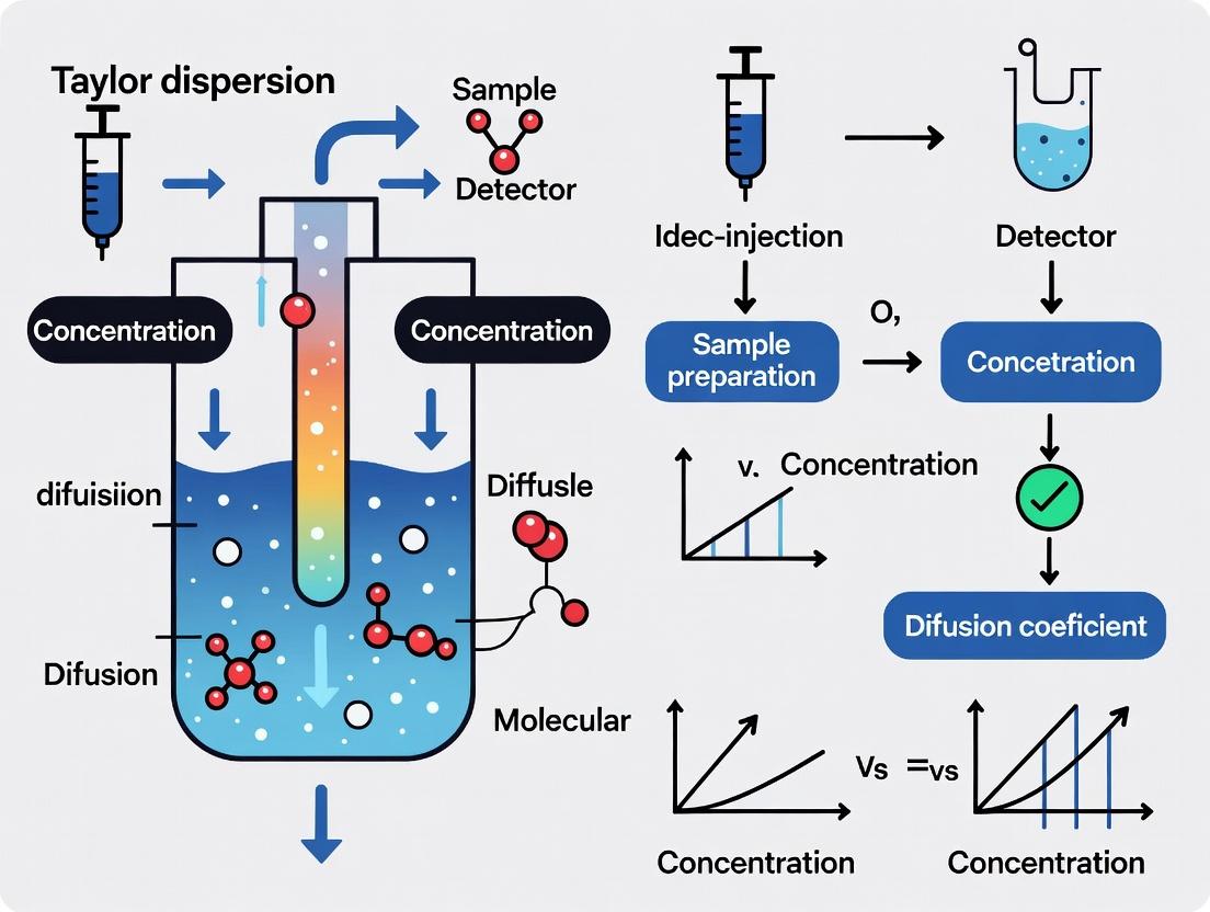
Visualization of Key Concepts

Diagram 1: Core Process & Binding Assay Workflow

Diagram 2: Evolution Timeline of the Technique

The Scientist's Toolkit

Table 2: Essential Research Reagent Solutions & Materials

Item	Function in Experiment	Key Specifications/Notes
Fused Silica Capillary	Conduit for laminar flow and dispersion.	Internal diameter: 10-75 µm. Coated to prevent analyte adsorption (e.g., PVA, polyimide).
High-Precision Syringe Pump	Generates pulseless, laminar flow.	Flow rate stability < 0.5% RSD in nL/min range. Critical for reproducible dispersion.
Thermostated Cartridge	Maintains constant temperature.	Temperature control ± 0.1 °C. Essential as D is temperature-dependent.
On-line Fluorescence Detector	Monitors dispersed peak in real-time.	High sensitivity for low-concentration samples. Alternatively, UV/Vis or MS detector.
Running Buffer	Mobile phase for the system.	Must match sample solvent to avoid viscosity gradients. Filtered (0.22 µm) and degassed.
Analyte/Protein Standards	For system calibration and validation.	e.g., FITC, BSA, monoclonal antibodies with known D values.
Data Acquisition & Analysis Software	Records signal and fits dispersion model.	Custom (e.g., in-house Python/Matlab scripts) or vendor-specific (e.g., for FIDA instruments).
Microfluidic Injection Valve	Introduces a precise, small sample plug.	Nanolitre injection volume capability with minimal dead volume.

Application Note: Taylor-Aris dispersion is a powerful hydrodynamic method for measuring the diffusion coefficients (D) of molecules in solution, critical for understanding solute-solvent interactions, molecular sizing, and binding kinetics in drug development. This note details the theoretical linkage and practical protocols within a thesis focused on advancing this measurement technique.

Theoretical Linkage: Flow, Dispersion, and D

In a pressure-driven laminar flow through a capillary, a parabolic velocity profile develops. A discrete solute plug is simultaneously stretched by the flow (convective dispersion) and blurred by molecular diffusion (D). The effective axial dispersion coefficient ((K)) is described by the Taylor-Aris equation: [ K = D + \frac{u^2 dc^2}{192D} ] where (u) is the average flow velocity and (dc) is the capillary diameter. Under conditions of slow flow and sufficient diffusion time, the second term dominates, creating a direct relationship between the observed peak variance ((\sigma_t^2)), measured via a concentration detector (e.g., UV), and D.

Table 1: Key Quantitative Relationships in Taylor Dispersion

Parameter	Symbol	Relationship to D	Typical Units
Effective Dispersion Coefficient	(K)	(K \approx \frac{u^2 d_c^2}{192D})	m²/s
Temporal Peak Variance	(\sigma_t^2)	(\sigma_t^2 = \frac{2K L}{u^3})	s²
Plate Height	(H)	(H = \frac{2K}{u})	m
Péclet Number	(Pe)	(Pe = \frac{u d_c}{D}) (Condition: (Pe > 70))	Dimensionless

Experimental Protocol: Determining D for a Small Molecule API

This protocol outlines the determination of the diffusion coefficient for a model Active Pharmaceutical Ingredient (API) using a capillary flow system coupled to a UV detector.

Materials & Preparation:

• Stock Solution: Prepare a 1.0 mg/mL solution of the API in phosphate-buffered saline (PBS), pH 7.4.
• Mobile Phase: Filtered and degassed PBS, pH 7.4.
• System: A syringe pump capable of stable, pulseless flow, a 5-meter long, 75 µm internal diameter fused silica capillary, a UV/VIS detector with a micro-flow cell, and a data acquisition system.

Procedure:

• System Equilibration: Flush the capillary thoroughly with mobile phase. Set the syringe pump to a constant flow rate (e.g., 1.0 µL/min, corresponding to (u \approx 3.77) mm/s) and allow pressure and detector baseline to stabilize for 30 minutes.
• Sample Injection: Using a six-port injection valve, introduce a 10 nL plug of the API stock solution into the flow stream.
• Data Acquisition: Record the detector output (voltage vs. time) at high temporal resolution as the dispersed sample plug passes through. Ensure the peak is fully captured and returns to baseline.
• Peak Analysis: Fit the resulting Gaussian-shaped peak profile. Precisely calculate the temporal variance ((\sigmat^2)) of the peak. For a Gaussian, (\sigmat^2 = (w{0.5})^2 / (8\ln2)), where (w{0.5}) is the peak width at half-height.
• Calculation of D: Using the known values of (L) (capillary length), (u), and (dc), calculate D by solving the combined equation: [ D = \frac{dc^2 u^2}{192 \left( \frac{\sigmat^2 u^3}{2L} - D \right)} ] An iterative approach is typically used, as D appears on both sides. Initial guess: (K = \frac{\sigmat^2 u^3}{2L}).
• Validation: Repeat measurements (n=5) at two different flow rates (e.g., 0.8 and 1.2 µL/min) to confirm that D is constant (flow-independent), validating that Taylor dispersion conditions were met.

The Scientist's Toolkit: Key Research Reagent Solutions & Materials

Table 2: Essential Materials for Taylor Dispersion Experiments

Item	Function & Importance
Fused Silica Capillary (ID: 50-100 µm)	Provides a uniform, narrow-bore conduit for laminar flow generation. Small (d_c) is critical to minimize the required dispersion length.
High-Precision Syringe Pump	Generates pulse-free, constant volumetric flow. Flow stability is paramount for accurate (\sigma_t^2) measurement.
UV/VIS Absorbance Detector	Quantifies solute concentration at the capillary outlet. Must have a low-dispersion, small-volume flow cell.
Precision Injection Valve	Enables reproducible introduction of nanoliter-scale sample plugs. A key source of experimental variance if not precise.
Standard Reference Compounds	Molecules with known, literature-reported D (e.g., potassium dichromate, bovine serum albumin) for daily system calibration and validation.
Degassed & Filtered Buffer	Mobile phase free of bubbles and particles prevents flow instability, pressure fluctuations, and capillary blockage.

Workflow and Relationship Diagrams

Diagram 1: Experimental Workflow for D Measurement

Diagram 2: Logical Path from Raw Data to D Value

The diffusion coefficient (D) is a fundamental physicochemical parameter that quantifies the rate at which a particle moves through a medium due to random thermal motion. In the context of biomolecular analysis, D provides critical, label-free insights into hydrodynamic size, conformational changes, oligomeric state, and binding interactions. Its measurement is indispensable for characterizing proteins, nucleic acids, lipids, and their complexes in solution under native conditions. This application note frames the importance of D within ongoing thesis research focused on advancing the Taylor Dispersion Analysis (TDA) method for robust, high-precision diffusion coefficient measurement. TDA offers distinct advantages for precious or challenging samples, including small volume requirements, minimal surface interaction, and compatibility with diverse buffers.

The Quantitative Link Between D, Size, and Shape

The Stokes-Einstein equation provides the foundational relationship between the translational diffusion coefficient (D_t) at infinite dilution and hydrodynamic radius (R_h): D_t = k_BT / 6πηR_h where k_B is Boltzmann’s constant, T is temperature, and η is solvent viscosity. Deviations from a spherical shape are quantified using the frictional ratio (f/f₀), derived from D. For macromolecules, D is inversely proportional to the cube root of molecular weight (M_w), providing a sensitive measure of oligomerization.

Table 1: Relationship Between Diffusion Coefficient, Hydrodynamic Size, and Molecular Parameters

Biomolecule	Approx. Mw (kDa)	Theoretical Rh (nm)	Typical D (10-7 cm²/s)	Key Insight from D
Lysozyme	14.3	1.9	11.0	Monomeric state benchmark
IgG1 Antibody	150	5.2	4.1	Hydrodynamic size for quality control
BSA (monomer)	66.5	3.5	6.0	Conformational stability
DNA (100 bp)	~66	4.8*	4.4*	Length & rigidity probe
Lipid Nanodisc	~200 (complex)	~5.5	~3.8	Size homogeneity assessment

*Values are illustrative; exact D depends on buffer, temperature, and conformation.

Application Notes: Deriving Biomolecular Insights from D

A. Assessing Oligomeric State and Aggregation

Changes in D are a direct indicator of changes in hydrodynamic size. A decrease in D (increase in R_h) signals dimerization/oligomerization or aggregation. This is vital for therapeutic protein development to monitor unwanted self-association.

Table 2: D as a Sensor for Oligomerization

Sample Condition	Expected Δ in D	Interpretation
Stable Monomer	Baseline (e.g., 11.0 x 10-7 cm²/s)	Reference state
Dimer Formation	Decrease by ~20%	Non-covalent self-association
Subvisible Aggregate	Decrease by >50%	Presence of multimers
Heat-Stressed Protein	Broadened D distribution	Heterogeneous aggregation

B. Characterizing Binding Interactions & Affinity

Monitoring D during titration of a ligand (small molecule, another protein) allows calculation of binding constants. The shift in D for the larger binding partner (e.g., a protein) upon complex formation reports on stoichiometry and affinity (K_D).

C. Probing Conformational Changes

Proteins undergoing folding/unfolding or domain rearrangements exhibit changes in R_h detectable via D. A more compact state has a higher D than an unfolded state of the same molecular weight.

Detailed Protocol: Taylor Dispersion Analysis for Diffusion Coefficient Measurement

Principle: A small bolus of sample is injected into a capillary containing a flowing background buffer. As it flows, the sample disperses axially due to flow velocity profile and radially due to diffusion. The resultant concentration profile at the detector (UV or fluorescence) is fitted to extract D.

Protocol: TDA of a Monoclonal Antibody

I. Research Reagent Solutions & Essential Materials Table 3: Scientist's Toolkit for TDA

Item	Function
Taylor Dispersion Instrument (e.g., dedicated system or modified HPLC/CE)	Precise fluidic handling, injection, and detection.
Fused Silica Capillary (50 µm ID, 50-100 cm length)	Laminar flow chamber for dispersion.
High-Precision Syringe Pump	Generates stable, pulse-free flow (typical range: 1-10 µL/min).
UV/Vis or Fluorescence Detector	Monitors dispersed sample zone.
Degassed, Filtered Background Buffer (e.g., PBS, pH 7.4)	Matches sample solvent; defines medium viscosity (η).
Sample (e.g., 1-2 mg/mL mAb) in background buffer	Analytic of interest; must be at known concentration.
Viscosity Standard (e.g., 1 mg/mL BSA)	Validates system performance and temperature control.
Data Acquisition and Analysis Software	Records dispersion profiles and fits data to Taylor model.

II. Step-by-Step Procedure

• System Preparation: Flush capillary extensively with background buffer. Set temperature control to 25.0 ± 0.1 °C. Precisely measure capillary length and inner diameter.
• Viscosity Calibration: Inject a standard (e.g., BSA with known D) at a defined flow rate (e.g., 2 µL/min). Record the dispersion profile (concentration vs. time).
• Sample Measurement: Inject sample bolus (typically 10-30 nL). Repeat at the same flow rate as calibration. Perform replicates (n≥3).
• Data Analysis: Fit the dispersion profile (a Gaussian-like peak) to the Taylor equation: C(t) = (C₀/√(4πD*t)) * exp(-(t₀ - t)²/(4D*t)) (adjusted for flow parameters). The variance (σ²) of the peak is linearly related to the capillary transit time and inversely related to D: σ² = (r²/(24D)) * t where r is capillary radius.
• Calculation: Use software to extract D from the fitted parameters. Normalize D to standard temperature and solvent (usually water at 20.0°C, D_20,w) using known viscosity/temperature relationships.

III. Critical Notes:

• Ensure flow is purely laminar (low Reynolds number).
• Injection volume must be optimized to avoid overloading.
• Buffer matching is critical to avoid viscosity gradients.
• For binding studies, pre-incubate complexes to equilibrium before injection.

Visualizing Concepts and Workflows

Title: How D Informs Biomolecular Properties & Applications

Title: Taylor Dispersion Analysis Experimental Workflow

Within the framework of a thesis investigating the Taylor Dispersion Analysis (TDA) method for diffusion coefficient (D) determination, this application note delineates the core operational advantages of the technique. TDA, which measures analyte dispersion within laminar flow in a capillary, is distinguished by its minimal sample demand, exceptional size range, and streamlined preparation. These attributes position it as a critical tool for the characterization of biomolecules and nanoparticles in drug development.

Core Advantages Quantified

The quantitative benefits of TDA are summarized in the following table, which contrasts it with traditional biophysical methods.

Table 1: Comparative Analysis of TDA with Traditional Characterization Techniques

Feature	Taylor Dispersion Analysis (TDA)	Dynamic Light Scattering (DLS)	Analytical Ultracentrifugation (AUC)
Sample Volume	5-20 µL	50-1000 µL	300-450 µL
Size Range (Hydrodynamic Radius, Rₕ)	0.1 nm – 500 nm	~1 nm – 10 µm	~1 nm – 10 µm
Sample Preparation	Minimal; often direct from formulation buffer. Filtration optional.	Often requires dilution; sensitive to dust, requiring filtration.	Requires precise loading; often needs buffer matching.
Concentration Range	Broad; µM to mM (UV detection)	Optimal at low concentrations to avoid aggregation.	Broad, but signal intensity dependent.
Measurement Time	5-15 minutes per run	2-5 minutes per run	Several hours to days
Primary Output	Diffusion Coefficient (D), Rₕ, Polydispersity	Rₕ, Size Distribution, Polydispersity	Sedimentation Coefficient, Molecular Weight, Purity

Detailed Application Notes & Protocols

Application Note 1: High-Throughput Screening of mAb Formulation Stability

• Objective: Rapidly assess the effect of 24 different excipient conditions on the colloidal stability of a monoclonal antibody (mAb) over 4 weeks at 40°C.
• TDA Advantage Utilization: The micro-volume requirement (10 µL per condition per time point) enables the entire study from a single, precious 5 mL starting material. Minimal preparation allows direct sampling from stress vials.
• Protocol:
  • Prepare mAb sample at 10 mg/mL in a base buffer.
  • Aliquot into 24 microcentrifuge tubes and add excipients (e.g., salts, sugars, surfactants) to final target concentrations.
  • Filter all samples through a 0.22 µm membrane filter into separate HPLC vials.
  • Place vials in a stability chamber at 40°C.
  • At t=0, 1, 2, and 4 weeks, remove vials and cool to room temperature.
  • For TDA analysis: Load a 75 cm fused silica capillary (75 µm ID) conditioned with running buffer (e.g., 20 mM Histidine-HCl, pH 6.0).
  • Set instrument parameters: Temperature = 25.0°C, Flow Rate = 1.0 µL/min, Injection Time = 30 s, UV Detection at 280 nm.
  • For each sample, flush capillary with running buffer for 3 min, perform a blank run with buffer, then inject the stressed mAb formulation.
  • Analyze the resulting Taylorgram using proprietary software to extract the diffusion coefficient (D) and calculate the hydrodynamic radius (Rₕ via the Stokes-Einstein equation).
  • Plot Rₕ vs. time for each formulation. A significant increase (>0.5 nm) indicates aggregation onset.

Application Note 2: Sizing of Polydisperse Lipid Nanoparticles (LNPs)

• Objective: Characterize the size distribution of a raw LNP formulation containing siRNA without dilution.
• TDA Advantage Utilization: The broad size range (1-500 nm) captures the core LNP population and potential large aggregates. Minimal preparation avoids shear or dilution-induced artifacts.
• Protocol:
  • Obtain LNP formulation post-extrusion. No dilution is performed unless concentration exceeds detector linear range (verify with a dilution series).
  • If necessary, gently invert the vial to homogenize without creating foam.
  • Load a 50 cm capillary (100 µm ID) conditioned with a diluent matching the LNP external phase (e.g., 1x PBS).
  • Set instrument parameters: Temperature = 25.0°C, Flow Rate = 0.8 µL/min, Injection Time = 45 s, UV Detection at 260 nm (for siRNA cargo).
  • Perform a buffer blank run.
  • Inject the native LNP formulation. The Taylorgram will be fitted to a multi-component dispersion model.
  • The software deconvolutes the signal to provide the diffusion coefficient and relative mass fraction for each detectable population (e.g., monomeric LNPs, oligomers, large aggregates).
  • Report the intensity-weighted mean Rₕ and the polydispersity index (PdI) derived from the distribution.

Visualization of Workflows

TDA Core Measurement Process

TDA Role in a Research Thesis

The Scientist's Toolkit: Research Reagent Solutions

Table 2: Essential Materials for TDA Experiments

Item	Function & Rationale
Fused Silica Capillary (e.g., 50-100 µm ID x 50-75 cm)	The core flow cell where Taylor dispersion occurs. Small internal diameter minimizes sample mixing via convection, ensuring dispersion is diffusion-controlled.
Precision Syringe Pump	Generates pulseless, laminar flow at low rates (µL/min). Flow stability is critical for reproducible Taylorgram generation.
High-Sensitivity UV/Vis Detector	Measures the concentration profile of the dispersed analyte plug. Required for detecting low-concentration samples in micro-volumes.
Thermostatted Capillary Cartridge	Maintains precise temperature (±0.1°C) to control solution viscosity and ensure accurate D measurement, as D is temperature-dependent.
In-line Degasser	Removes dissolved gases from running buffers to prevent bubble formation in the capillary, which disrupts flow and detection.
0.22 µm or 0.1 µm Membrane Filters (PES or PVDF)	For clarifying running buffers and samples. Removes particulates that could block the capillary or create noise.
Certified Vials & Low-Volume Inserts	Minimizes sample dead volume and adsorption for precious, low-volume samples.
Standard Reference Materials (e.g., BSA, sucrose)	Used for daily system calibration and validation to ensure accuracy of diffusion coefficient measurements.

Step-by-Step Protocol: Implementing Taylor Dispersion Analysis in Your Lab

This application note details the essential instrumentation and protocols for conducting diffusion coefficient (D_t) measurements via the Taylor dispersion method, a core analytical technique within the broader thesis research "Advanced Hydrodynamic Characterization of Biotherapeutics in Solution." Accurate D_t values are critical for determining hydrodynamic radius, assessing protein self-association, and characterizing formulation stability in drug development.

Core Equipment Components & Specifications

Capillaries

The capillary is the central component where Taylor dispersion occurs. Its dimensions and quality directly impact measurement accuracy.

Table 1: Capillary Specifications and Selection Criteria

Parameter	Specification	Rationale
Material	Fused silica with polyimide coating	Chemically inert, provides mechanical strength, allows for optical detection windows.
Inner Diameter (ID)	50 - 150 µm (75 µm optimal for most proteins)	Balances sufficient sample volume with high radial dispersion efficiency. A smaller ID reduces the required axial length for full development of the Taylor regime.
Length	1 - 10 m (typically 2-5 m coiled)	Provides adequate length for complete axial dispersion of the sample plug and establishment of a parabolic flow profile.
Temperature Control	Must be housed in a thermostated compartment (±0.1 °C)	Diffusion coefficient is highly temperature-sensitive (≈2-3% per °C). Precise control is non-negotiable.

Pumps & Flow Systems

A pulse-free, highly stable flow delivery system is required to maintain a constant Poiseuille flow profile.

Protocol 1.1: Pump Calibration and Flow Rate Optimization

• Equipment Setup: Connect a high-precision, dual-syringe HPLC or dedicated capillary flow pump to the capillary inlet via low-dead-volume fittings. Install a calibrated flow sensor at the outlet for verification.
• Flow Rate Calibration: At a constant temperature (e.g., 25.0 °C), set the pump to deliver a series of flow rates (e.g., 0.5, 1.0, 2.0 µL/min). Collect effluent in a pre-weighed vial over a precise time (10 min). Calculate actual flow rate from mass difference (assuming density = 1.00 g/mL for aqueous buffers).
• Optimal Flow Determination: The optimal flow rate (Q_opt) balances Taylor condition (sufficiently slow flow) and detection sensitivity. A starting point is calculated using: Q_opt ≈ (3000 * π * D_t * r^3) / L, where r is capillary radius, L is length, and D_t is an estimated diffusion coefficient. Empirically test rates between 0.5 and 5 µL/min.
• Validation: Inject a standard (e.g., 1 mg/mL BSA in PBS) and analyze the resulting peak shape. The peak should be symmetrical and fit well to the Taylor dispersion model (see Software section). Adjust flow rate until optimal fit (R² > 0.99) is achieved.

Detectors

Detection occurs directly on-capillary. UV/Vis absorbance is most common, but fluorescence and refractive index (RI) are also used.

Table 2: Detector Performance Comparison

Detector Type	Typical Noise Level	Concentration Sensitivity	Key Advantage	Key Limitation
UV/Vis Absorbance	± 0.0001 AU	~0.1 mg/mL (for A280)	Universal for proteins/peptides; robust.	Requires chromophore; lower sensitivity than fluorescence.
Fluorescence	± 0.001 FU	~1-10 µg/mL (for Trp emission)	Extremely high sensitivity and selectivity.	Requires fluorophores; potential for photobleaching.
Refractive Index (RI)	± 1.0e-8 RI units	~0.5 mg/mL	Universal detection; no label required.	Highly sensitive to temperature and pressure fluctuations.

Protocol 1.2: Detector Wavelength Selection & Baseline Optimization

• For UV/Vis: Prior to sample runs, perform a blank buffer (carrier phase) injection at the intended detection wavelength (typically 280 nm for proteins, 214 nm for peptides). Record the baseline for at least 10 column volumes.
• Baseline Criteria: A stable baseline is critical. The peak-to-peak noise should be < 0.0005 AU over 5 minutes. If noise is high, ensure sufficient lamp warm-up time (>30 min), purge the flow cell with buffer, and verify thermostatting.
• For Fluorescence: Set excitation/emission wavelengths appropriate for the analyte (e.g., Ex 280 nm / Em 350 nm for tryptophan). Use appropriate filters to minimize scattered light. Perform a blank injection to confirm absence of background fluorescence from the buffer or capillary.

Software & Data Analysis

Software is required for instrument control, data acquisition, and, most critically, non-linear regression fitting of the dispersion profile to extract D_t.

Protocol 1.3: Data Acquisition and Analysis Workflow

• Acquisition: Using instrument control software (e.g., Clarity, ChromScope), set a high data acquisition rate (≥ 10 Hz) to adequately define the dispersion peak shape. Configure the injection time (typically 1-5 seconds) to define the initial plug length.
• Pre-processing: Export the raw detector signal (time, intensity). Subtract a linear baseline fitted to the pre- and post-peak regions. Normalize the peak maximum to 1.
• Non-Linear Regression: Fit the normalized data to the Taylor-Aris equation: C(t) = C0 * sqrt(tD / (t^3)) * exp( - (t0 - t)^2 * tD / (t^3) ) where C(t) is concentration at time t, t₀ is the mean residence time, and t_D is the characteristic dispersion time related to D_t.
• Calculation: Calculate the diffusion coefficient using: D_t = (r^2) / (24 * t_D), where r is the capillary inner radius. Report the average and standard deviation of at least three independent injections.

Integrated Experimental Workflow

Diagram 1: Taylor Dispersion Experiment Workflow

The Scientist's Toolkit: Research Reagent Solutions

Table 3: Essential Materials for Taylor Dispersion Experiments

Item	Function & Specification	Example Product/Catalog Number (for informational purposes)
Fused Silica Capillary	The dispersion column. 75 µm ID, 360 µm OD, 3-5 m length, polyimide coated.	Polymicro TSP075375, Molex 1068150001
Capillary Flanges/ Ferrules	For leak-free, low-dead-volume connection to the injector and detector. Must match capillary OD and fitting type (e.g., 1/4-28 or 10-32).	Idex Health & Science F-126, P-720
High-Precision Syringe Pump	Generates pulse-free, constant flow of carrier buffer.	Teledyne CETONI neMESYS, Chemyx Fusion 7500
Micro-Injection Valve	Provides reproducible, timed injections of sample plug into the capillary.	Rheodyne 7725i (with 0.5 µL internal loop)
UV/Vis Flow Cell Detector	Measures absorbance of the dispersed sample plug directly in the capillary.	Knauer Azura UVD 2.1S (with capillary flow cell)
Thermostated Compartment	Maintains constant temperature for capillary, pump head, and detector cell.	Custom-built oven or column heater (e.g., BASi 402100)
Protein Standard (BSA)	Used for system validation and calibration. Lyophilized, ≥98% purity.	Sigma-Aldrich A7906
PBS Buffer, Molecular Biology Grade	Standard carrier phase for biomolecule studies. Filtered (0.1 µm) and degassed.	Gibco 10010-023
Data Acquisition & Analysis Software	Controls hardware and performs non-linear regression fitting of dispersion data.	Clarity Chromatography Software, self-coded routines in Python/Matlab.
0.1 µm In-line Filter	Placed between buffer reservoir and pump to prevent capillary clogging.	Upchurch Scientific A-101X

Sample Preparation Best Practices for Proteins, mRNAs, LNPs, and Viscous Solutions

Within the broader thesis on Taylor dispersion method (TDA) diffusion coefficient (D) measurement research, rigorous sample preparation is the critical determinant of data fidelity. The measured D is exquisitely sensitive to sample aggregation, conformational changes, and contaminants. This application note details protocols optimized for TDA analysis of complex biologics and formulations, ensuring minimal perturbation and accurate hydrodynamics-based characterization.

Sample-Specific Preparation Protocols

Proteins (Monoclonal Antibodies, Enzymes)

Objective: To prepare monodisperse, native, and stable protein samples for D measurement, preventing self-association or surface adsorption.

Detailed Protocol:

• Buffer Exchange: Employ centrifugal filtration (e.g., 10 kDa MWCO Amicon filters) or dialysis into the desired analysis buffer (e.g., PBS, Histidine buffer). Perform three buffer exchanges at 4°C to ensure complete replacement.
• Clarification: Centrifuge the protein solution at 14,000-16,000 x g for 10 minutes at 4°C to remove any large aggregates or insoluble particles. Carefully pipette the supernatant without disturbing the pellet.
• Concentration Adjustment: Dilute or concentrate (using centrifugal filtration) the protein to the target concentration range for TDA (typically 0.1-2 mg/mL). Avoid overshooting concentration to prevent aggregation.
• Filtration: Immediately prior to TDA injection, pass the sample through a 0.22 µm or 0.1 µm low-protein-binding syringe filter (e.g., PVDF or cellulose acetate).
• Handling: Keep samples on ice or at 4°C and analyze within 2 hours of final preparation.

Messenger RNA (mRNA)

Objective: To prepare intact, non-degraded mRNA samples, free of aggregates that could skew diffusion analysis.

Detailed Protocol:

• Thawing: Rapidly thaw frozen mRNA stock on wet ice. Do not use heat or repeated freeze-thaw cycles.
• Buffer Compatibility: Ensure the mRNA is in a nuclease-free, low-ionic-strength buffer (e.g., 1 mM sodium citrate, pH 6.5). If necessary, perform buffer exchange using RNase-free centrifugal filters (e.g., 100 kDa MWCO).
• Denaturation Control: For D measurements intended to assess the folded state, heat the sample to 70°C for 2 minutes, then snap-cool on ice to standardize secondary structure. For native conditions, omit this step.
• Aggregate Removal: Centrifuge at 12,000 x g for 5 minutes at 4°C. Transfer supernatant to a new RNase-free tube.
• Final Preparation: Dilute to the required concentration (typically 0.05-0.5 mg/mL) using nuclease-free buffer. Analyze immediately.

Lipid Nanoparticles (LNPs)

Objective: To prepare a homogeneous, non-sedimenting LNP dispersion representative of the bulk formulation for accurate size and D measurement.

Detailed Protocol:

• Equilibration: Allow the LNP formulation to equilibrate to the analysis temperature (e.g., 20°C or 25°C) for at least 30 minutes. Gently invert the vial 10 times to ensure mixing. Do not vortex.
• Dilution: Dilute the LNPs in the exact same buffer as the formulation (e.g., Tris-sucrose buffer) to achieve a final particle concentration suitable for TDA (typically 1e10-1e11 particles/mL). Dilution is critical to minimize multiple scattering and particle interactions. Use serial dilution for accuracy.
• Homogenization: Gently mix the diluted sample by inverting the tube 5-10 times.
• Direct Injection: Load the sample into the TDA instrument without filtration or centrifugation, which can disrupt or fractionate the LNP population.

Viscous Solutions (Polymers, High-Concentration Proteins)

Objective: To ensure homogeneity and eliminate air bubbles, which create major artifacts in TDA due to mismatched viscosity and dispersion profiles.

Detailed Protocol:

• Degassing: Prior to dilution or use, degas the bulk viscous solution or buffer under mild vacuum with gentle stirring for 15-30 minutes.
• Mixing: For solutions of non-shear-sensitive polymers, use slow-speed vortex mixing. For high-concentration proteins, use gentle pipette mixing or end-over-end rotation.
• Centrifugation: Centrifuge samples in low-adhesion microcentrifuge tubes at 5,000-10,000 x g for 10-20 minutes to sediment any micro-bubbles or particulates.
• Loading: Pipette the sample slowly and carefully from the center of the tube, avoiding the top (air interface) and bottom (pellet). Allow the sample to thermally equilibrate in the instrument capillary for 5 minutes before starting the run.

Sample Type	Ideal Conc. for TDA	Critical Buffer Component	Key Preparation Step	Stability Window Post-Prep	Dominant Artifact Risk
Proteins	0.1 - 2 mg/mL	Surfactant (e.g., 0.01% PS-80)	0.1 µm Filtration	2-4 hours at 4°C	Aggregation, Surface Adsorption
mRNAs	0.05 - 0.5 mg/mL	Nuclease-free Water, 1 mM Citrate	Heat-Snap Cool (if needed)	<1 hour on ice	RNase Degradation, Aggregation
LNPs	1e10 - 1e11 part./mL	Iso-osmotic Sucrose/Tris	Minimal Gentle Mixing	Immediate Analysis	Sedimentation, Fusion
Viscous Solutions	Dilute to < 10x Buffer Viscosity	Matching Solvent	Degassing & Slow Centrifugation	1 hour	Microbubbles, Inhomogeneity

The Scientist's Toolkit: Key Reagents & Materials

Item	Function in TDA Sample Prep
Amicon Ultra Centrifugal Filters	Buffer exchange and concentration of proteins/mRNAs; removes small molecule impurities.
Low-Protein-Binding Syringe Filters (0.1 µm PVDF)	Sterile filtration of protein solutions to remove particulates and aggregates without adsorption.
Nuclease-Free Microcentrifuge Tubes & Tips	Prevents degradation of RNA samples during handling and preparation.
Formulation-Matched Blank Buffer	Essential for LNP dilution and as the reference dispersion medium in TDA; ensures no osmotic shock.
Degassing Station (Vacuum Chamber)	Removes dissolved air from viscous solutions to prevent bubble formation in the capillary.
Precision Positive-Displacement Pipettes	Accurate handling of viscous samples where air-displacement pipettes fail.
Chemical-Compatible Vial Inserts	Prevents leaching of contaminants from sample vials for sensitive formulations.

Experimental Workflow & Conceptual Diagrams

Title: TDA Sample Prep Workflow for Four Biologic Types

Title: Role of Sample Prep in TDA Thesis & Applications

Within the broader thesis on advancing the Taylor dispersion method for diffusion coefficient (D) measurement, this document details the critical experimental phase of solute injection and flow parameter establishment. Accurate D determination hinges on a perfectly controlled initial condition (a sharp, reproducible solute pulse) and stable, predictable laminar flow within the capillary. This protocol focuses on the practical execution of these parameters and the precise acquisition of temporal concentration data, which forms the primary dataset for analysis.

Experimental Protocols

Protocol 2.1: System Preparation and Capillary Conditioning

Objective: To ensure a contamination-free, stable fluidic system with reproducible surface properties.

• Flush the entire flow path (injection valve, capillaries, connectors, detection cell) with purified water (HPLC grade) for 10 minutes at a high flow rate (e.g., 1 mL/min) using a high-precision syringe pump.
• Condition the capillary with the chosen carrier buffer (e.g., 10 mM phosphate buffer, pH 7.4) for 20 minutes at the experimental flow rate.
• Verify system stability by monitoring the baseline signal from the UV/Vis or fluorescence detector for at least 15 minutes. The baseline drift must be < 0.1 mAU/min.

Protocol 2.2: Optimization of Injection Pulse Shape

Objective: To generate a sharp, symmetrical solute plug.

• Prepare a stock solution of the analyte (e.g., 1 mg/mL bovine serum albumin in carrier buffer).
• Using a 6-port, 2-position injection valve with a fixed-volume sample loop (e.g., 10 µL):
  • Load the sample loop completely via a manual loading port or an auxiliary pump, ensuring no air bubbles.
  • Switch the valve from "Load" to "Inject" position for a precisely timed duration (t_inject).
  • Critical: For Taylor dispersion, t_inject must be short enough that the initial pulse width is negligible compared to the dispersed peak width. A rule of thumb: t_inject < 0.1 * t_peak (peak mean residence time). Start with t_inject = 1-2 seconds.
• The carrier stream immediately sweeps the sample plug into the capillary. The sharpness is evaluated by the resulting peak shape (see Protocol 2.4).

Protocol 2.3: Establishment and Verification of Laminar Flow

Objective: To achieve stable, parabolic (Hagen-Poiseuille) flow.

• Set the syringe pump to a constant flow rate (Q). For a typical 50 µm inner diameter (ID) fused silica capillary, start with Q = 10 µL/min.
• Calculate the Reynolds number (Re) to confirm laminar flow regime:
  • Re = (ρ * v * d) / η, where ρ = fluid density, v = flow velocity, d = capillary ID, η = dynamic viscosity.
  • For aqueous buffers in sub-mm capillaries, Re is typically << 100, ensuring laminar flow.
• Verify flow stability by performing 5 consecutive injections of a standard dye and measuring the retention time. The coefficient of variation (CV) of retention times must be < 0.5%.

Protocol 2.4: Temporal Data Acquisition and Peak Recording

Objective: To acquire high-fidelity concentration-time data (C(t)).

• Position the detector (e.g., UV/Vis) at a fixed distance (L) from the injection point. Record L precisely (± 0.1 cm).
• Set detector data acquisition rate to at least 10-20 Hz to adequately capture the peak shape.
• Trigger data acquisition synchronously with the valve switch to "Inject."
• Record the resulting dispersion peak until the signal returns to within 1% of the baseline.
• Save data in a non-proprietary format (e.g., .csv) with columns for Time (s) and Signal (mV or AU).

Data Presentation

Table 1: Summary of Critical Flow and Injection Parameters for Taylor Dispersion

Parameter	Symbol	Typical Value Range	Recommended Optimization Method	Impact on D Measurement
Capillary Inner Diameter	d	50 - 250 µm	Fixed by hardware choice.	Larger d enhances dispersion signal but requires higher Q for same t_peak.
Flow Rate	Q	5 - 100 µL/min	Sweep Q to validate linearity of σ² vs. t_peak.	Must be constant. Optimal range balances sufficient dispersion and experiment time.
Flow Velocity	v	1 - 20 cm/min	Calculated as v = 4Q / (πd²).	Directly determines residence time t_peak = L / v.
Injection Time	t_inject	1 - 5 s	Minimize until peak asymmetry > 5%.	Excessive t_inject adds non-dispersive peak broadening, causing overestimation of D.
Capillary Length to Detector	L	50 - 200 cm	Fixed, measure precisely.	Longer L increases dispersion magnitude, improving fitting accuracy.
Peak Mean Residence Time	t_peak	2 - 15 min	Calculated from recorded peak.	Core variable in Taylor equation: D = (d² * t_peak) / (96 * σ²).
Peak Temporal Variance	σ²	10 - 200 s²	Obtain from Gaussian fit of C(t) data.	Core variable. Must be corrected for finite injection volume contribution.

Table 2: Key Research Reagent Solutions & Materials

Item	Function	Critical Specifications
Fused Silica Capillary	Conduit for laminar flow and Taylor dispersion.	Inner diameter uniformity (± 1%), chemically inert, transparent for on-capillary detection.
High-Precision Syringe Pump	Generates pulseless, constant volumetric flow.	Flow rate accuracy and precision < ± 0.5%, low pulsation.
Micro-Volume Injection Valve	Introduces a sharp, discrete solute plug.	6-port/2-position, low dead volume (< 100 nL), electrically actuated for precise timing.
UV/Vis or Fluorescence Detector	Measures temporal concentration profile C(t).	High sensitivity, low noise, fast response time, small flow cell volume (< 1 µL).
Carrier Buffer	Matches sample matrix, defines solvent properties.	Filtered (0.22 µm), degassed, controlled pH and ionic strength to prevent analyte interactions.
Diffusion Standard (e.g., Potassium Dichromate)	Validates experimental setup and data processing.	Known, literature-reported D value in the used buffer at a specific temperature.

Mandatory Visualizations

Experimental Workflow for Taylor Dispersion Measurement

Physics of Taylor Dispersion: Flow & Peak Broadening

Within the broader thesis on advancing the Taylor dispersion method for diffusion coefficient measurement, this protocol focuses on the critical data analysis phase. The accurate extraction of the diffusion coefficient (D) and the subsequent calculation of the hydrodynamic radius (R_h) from the raw dispersion profile is paramount for characterizing biomolecules, nanoparticles, and therapeutics in drug development.

Core Theory & Data Fitting Equation

In Taylor dispersion analysis (TDA), a sample plug is injected into a laminar flow of carrier fluid within a capillary. The combination of parabolic flow velocity and radial diffusion results in a characteristic concentration profile at the detector (typically UV or fluorescence). The temporal profile can be fitted to the following equation to extract D:

Equation 1: Dispersion Profile C(t) = C₀ + ΔC \sqrt{\frac{t_0}{t}} \exp\left[ -\frac{2D(t - t_0)^2}{w^2 t} \right]

Where:

• C(t): Detected concentration at time t.
• C₀: Baseline signal.
• ΔC: Signal amplitude.
• t₀: Mean residence time of the sample plug.
• w: A dispersion parameter related to capillary geometry and flow.

The hydrodynamic radius is then calculated using the Stokes-Einstein equation:

Equation 2: Stokes-Einstein R_h = \frac{k_B T}{6 \pi \eta D}

Where:

• k_B: Boltzmann constant (1.380649 × 10^-23 J·K^-1).
• T: Absolute temperature (K).
• η: Dynamic viscosity of the solvent (Pa·s).
• D: Diffusion coefficient (m²·s^-1).

Experimental Protocol: TDA Measurement for Data Acquisition

Objective: To acquire a high-fidelity dispersion profile of a sample for subsequent fitting.

Materials & Instrumentation:

• Taylor Dispersion Instrument (e.g., dedicated TDA system or modified HPLC/CE system).
• Fused silica capillary (length: 1-10 m, internal diameter: 50-150 µm).
• Precision syringe pump for carrier stream.
• Injection valve (nanolitre volume).
• On-capillary UV/Vis or fluorescence detector.
• Temperature-controlled compartment.
• Data acquisition software.

Procedure:

• System Equilibration: Fill the capillary with filtered (0.1 µm) carrier buffer (e.g., PBS, 10 mM phosphate). Set the temperature control to 25.0 ± 0.1 °C. Initiate laminar flow at a defined, stable velocity (typically 0.5 - 5 µL/min).
• Sample Preparation: Prepare the analyte (e.g., monoclonal antibody, protein, nanoparticle) in the same carrier buffer. Filter (if appropriate) and degas.
• Injection: Using a calibrated injection loop or valve, introduce a narrow plug (10-100 nL) of the sample into the capillary.
• Data Recording: Continuously record the detector signal at a high sampling rate (≥10 Hz) as the dispersed plug passes through. Record until the signal returns to baseline.
• Replication: Perform a minimum of three independent injections per sample to ensure reproducibility.
• System Calibration: Perform a control experiment with a standard of known D (e.g., bovine serum albumin, sucrose) to validate system performance and calibrate capillary parameters.

Data Analysis Protocol: Fitting the Profile

Objective: To fit the raw C(t) data to Equation 1 and extract D and R_h.

Software Requirements: A non-linear least squares fitting tool (e.g., Python with SciPy, MATLAB, Origin, GraphPad Prism).

Procedure:

• Data Pre-processing: Import the raw temporal data. Subtract the baseline signal (C₀). If necessary, apply a smoothing filter (Savitzky-Golay) to reduce high-frequency noise without distorting the profile.
• Initial Parameter Estimation:
  • t₀: Estimate as the time at the peak maximum.
  • ΔC: Estimate as the peak height.
  • w: Can often be held constant from a calibration run with a known standard.
  • D: Provide an initial guess based on sample type (e.g., 5×10^-11 m²/s for an IgG).
• Non-Linear Curve Fitting: Implement Equation 1 as the model function. Use a Levenberg-Marquardt algorithm to minimize the sum of squared residuals between the experimental data and the model.
• Quality Assessment: Examine the fitted curve overlay on the raw data. Analyze residuals (difference between data and fit) – they should be randomly distributed. Calculate the coefficient of determination (R²) and confidence intervals for the fitted parameters.
• Calculate R_h: Insert the fitted value of D (in m²/s) along with the experimental temperature (T) and the solvent viscosity (η) into Equation 2 to compute R_h.
• Error Propagation: Calculate the standard error for R_h by propagating the standard error of D and the uncertainties in T and η.

Data Presentation

Table 1: Example Fitting Results for Protein Standards (T = 25.0°C, η = 0.890 mPa·s)

Protein (Standard)	Expected D (10⁻¹¹ m²/s)	Fitted D ± SD (10⁻¹¹ m²/s)	Fitted Rh ± SD (nm)	R² of Fit
Lysozyme	11.0	10.9 ± 0.2	1.96 ± 0.04	0.9995
BSA	5.9	6.0 ± 0.1	3.57 ± 0.06	0.9998
IgG1 (mAb)	4.1	4.2 ± 0.2	5.10 ± 0.24	0.9993

Table 2: Key Research Reagent Solutions & Materials

Item	Function & Specification
Filtered Carrier Buffer	Provides the background electrolyte. Must be matched to sample buffer to avoid viscosity gradients. Filter through 0.1 µm to remove particulates.
Fused Silica Capillary	The dispersion chamber. Standard ID: 75 µm; Length: 3-5 m. Requires precise temperature control.
Diffusion Standards	Known D molecules (e.g., sucrose, BSA) for system calibration and validation of the fitting protocol.
Precision Syringe Pump	Generates a pulse-free, laminar carrier flow. Stability is critical for reproducible t0.
Nanolitre Injection Valve	Introduces a sharp, well-defined sample plug into the capillary. Typical volume: 50 nL.
On-capillary UV Detector	Monitors the dispersed sample concentration profile over time. High signal-to-noise ratio is essential.

Visualizations

Title: TDA Workflow from Injection to D

Title: Data Fitting Algorithm to Extract D and Rh

Thesis Context: This work details critical applications of Taylor Dispersion Analysis (TDA) for diffusion coefficient (Dt) measurement, supporting a broader thesis on TDA's superiority in characterizing hydrodynamic size and stability of complex biopharmaceuticals in their native state, without separation or labeling.

Application Notes

Taylor Dispersion Analysis (TDA) is a flow-based, absolute method for measuring the diffusion coefficient (Dt) of analytes in solution. The derived hydrodynamic radius (Rh) via the Stokes-Einstein equation provides a critical stability and quality attribute. TDA is uniquely suited for polydisperse, fragile, or complex formulations where light scattering or SEC may fail.

Monoclonal Antibodies (mAbs) & Bispecifics: Stability & Developability

TDA monitors mAb self-interaction and conformational changes under stress (thermal, pH, mechanical). A shift to lower Dt (higher Rh) indicates aggregation or swelling, while a shift to higher Dt suggests fragmentation. It is a key tool for screening formulation conditions and identifying optimal candidates with minimal propensity for viscous or unstable behavior.

Antibody-Drug Conjugate (ADC) Aggregation & Drug Loading Impact

Conjugation of hydrophobic payloads can induce aggregation. TDA quantifies the proportion of high-molecular-weight species (HMWs) and monitors conjugation-induced size changes in real-time, complementing drug-to-antibody ratio (DAR) analysis. It is essential for assessing batch-to-batch consistency and stability post-conjugation.

Virus-Like Particle (VLP) Integrity & Empty/Full Ratio

VLPs are complex, hollow structures. TDA sensitively differentiates between intact VLPs, broken particles, and free capsid proteins based on their distinct Dt values. It provides a rapid, quantitative measure of assembly efficiency and product homogeneity, critical for vaccine efficacy and manufacturing control.

Liposome & Lipid Nanoparticle (LNP) Stability & Size Distribution

TDA characterizes vesicle size, polydispersity, and stability under physiological conditions (e.g., in serum). It monitors drug leakage (which changes core viscosity and Dt) and particle fusion or degradation over time, providing crucial data for nanoparticle drug delivery system optimization.

Table 1: Quantitative Diffusion Data for Key Biopharmaceuticals

Analytic	Typical Dt (m²/s)	Derived Rh (nm)	Key Stability Indicator	Stress Condition Monitored
IgG1 mAb (native)	~4.0 × 10⁻¹¹	~5.2	Dt decrease >5%	Thermal (40-60°C), agitation
ADC (DAR 4)	~3.8 × 10⁻¹¹	~5.5	Population at Dt < 3.5×10⁻¹¹	Storage (2-8°C, long-term)
VLP (intact, 30nm)	~1.5 × 10⁻¹¹	~14.0	Main peak Dt fidelity	Freeze-thaw, pH shift
siRNA-LNP	~2.0 × 10⁻¹²	~100.0	Dt distribution broadening	Serum incubation, 37°C

Table 2: TDA vs. Traditional Sizing Methods

Method	Sample Consumption	Analysis Time	Polydisperse Samples	Native State	Key Limitation for These Apps
Taylor Dispersion	Low (µL)	Fast (<10 min)	Excellent	Yes	Requires known analyte concentration
Dynamic Light Scattering	Low	Moderate	Poor	Yes	Sensitive to dust/aggregates
SEC-MALS	Moderate	Slow	Good	No (phase separation)	Shear-induced degradation, column interactions
Analytical Ultracentrifugation	High	Very Slow	Excellent	Yes	Low throughput, complex analysis

Experimental Protocols

Protocol 1: TDA Measurement for mAb/ADC Thermal Stability

Objective: Determine the onset temperature of aggregation and quantify aggregate formation.

Materials: See "The Scientist's Toolkit" below. Procedure:

• Sample Preparation: Dialyze mAb/ADC sample into formulation buffer (e.g., Histidine-Sucrose, pH 6.0). Filter using a 0.1 µm centrifugal filter. Determine precise concentration via UV absorbance (A280).
• Instrument Priming: Flush the TDA capillary system (75 µm i.d., ~10 m length) with filtered dialysate buffer at 0.5 µL/min for 30 min to establish baseline.
• Injection & Run: Perform a 20 nL controlled injection of sample. Initiate flow with a optimized, low-dispersion pump at a constant rate (typically 0.2-0.5 µL/min). Monitor elution via a high-sensitivity UV (or fluorescence) detector at 280 nm.
• Data Analysis: Fit the resulting dispersion profile (temporal variance of the concentration bell curve) to the Taylor equation: Dt = (uR²)/(24σ²). Where u is linear velocity, R is capillary radius, and σ² is temporal variance. Software converts Dt to Rh via Stokes-Einstein: Rh = (kT)/(6πηDt), where k is Boltzmann's constant, T is temperature, and η is buffer viscosity.
• Stress Study: Incubate aliquots at 25°C, 40°C, 50°C, and 60°C for 24 hours. Cool, centrifuge briefly, and analyze each via TDA. Plot Rh vs. incubation temperature.

Protocol 2: Assessing VLP Assembly Efficiency

Objective: Quantify the percentage of intact VLPs versus free protein or broken aggregates.

Materials: Purified VLP sample, reference buffer (e.g., PBS, pH 7.4), density gradient buffer. Procedure:

• Calibration: Run a standard of known Dt (e.g., a monoclonal antibody) to confirm system performance.
• Sample Analysis: Inject 30 nL of purified VLP preparation. Perform TDA run in triplicate.
• Data Deconvolution: Analyze the dispersion profile using a multi-Gaussian fitting algorithm. Identify peaks corresponding to: a) Large aggregates (Dt ~0.5-1.0×10⁻¹¹ m²/s), b) Intact VLPs (Dt ~1.5×10⁻¹¹ m²/s), c) Free capsid protein/dimers (Dt ~4.5×10⁻¹¹ m²/s).
• Quantification: Report the relative area-under-the-curve (%) for each peak, representing the population distribution. Intact VLP percentage >80% is typically target for vaccine candidates.

Protocol 3: Monitoring Liposome Serum Stability

Objective: Track liposome size increase or drug leakage in biologically relevant media.

Materials: Liposome formulation, 100% FBS, isotonic buffer (HBS, pH 7.4). Procedure:

• Baseline Measurement: Perform TDA on liposome sample diluted in HBS to a final lipid concentration of 0.1 mg/mL. Record mean Dt and distribution width.
• Serum Challenge: Mix liposome sample with pre-warmed FBS at a 1:1 (v/v) ratio. Incubate at 37°C.
• Time-Point Sampling: At t=0 (immediate mix), 30 min, 1h, 2h, 4h, and 24h, withdraw an aliquot. Dilute 10-fold into cold HBS to slow reaction. Centrifuge briefly to remove large serum aggregates if necessary.
• Analysis: Run TDA on each time-point aliquot. Plot mean hydrodynamic radius (Rh) versus time. A sharp increase indicates particle fusion/aggregation; a gradual shift may indicate swelling or drug leakage.

Diagrams

Title: TDA Core Experimental Workflow

Title: Biopharmaceutical Stress Pathways & TDA Detection

The Scientist's Toolkit: Key Research Reagent Solutions

Item	Function in TDA Experiments
Low-Protein-Binding Filters (0.1 µm)	Removes dust and pre-existing aggregates from samples and buffers, critical for baseline noise reduction.
High-Purity Dialysis Buffers (e.g., Histidine, Succinate, PBS)	Provides consistent, particle-free sample matrix with controlled ionic strength and pH for stability studies.
Diffusion Coefficient Standards (e.g., BSA, mAb, latex nanospheres)	Validates instrument performance and ensures accuracy of Dt measurements across different sizes.
Precision Syringe Pumps	Generates pulseless, ultra-low flow rates (µL/min) essential for creating reproducible laminar flow in the capillary.
High-Sensitivity UV/Vis Flow Cell Detector	Measures the subtle dispersion profile of the sample peak with high signal-to-noise ratio.
Viscosity Standard (e.g., Sucrose solutions)	Used for accurate determination of buffer viscosity (η), required for precise Rh calculation from Dt.
Temperature-Controlled Sample Chamber	Enables controlled stress studies (thermal stability) and ensures consistent temperature during analysis.
Multi-Gaussian Peak Fitting Software	Deconvolutes complex dispersion profiles from polydisperse samples (e.g., VLP mixtures, aggregating mAbs).

Solving Common TDA Challenges: A Troubleshooting and Optimization Guide

Identifying and Correcting for Instrumental Broadening and Background Noise

Within the broader thesis on Taylor dispersion method diffusion coefficient measurement research, accurate data extraction is paramount. The measured dispersion profiles are convolved with instrumental broadening effects and superimposed on background noise, which, if uncorrected, lead to significant systematic errors in the calculated diffusion coefficients (D). These coefficients are critical for characterizing biomolecular size, conformation, and interactions in drug development. This application note details protocols to identify, quantify, and correct for these artifacts.

Table 1: Common Sources of Instrumental Broadening and Noise in Taylor Dispersion

Source	Typical Magnitude/Effect	Impact on Calculated D
Detector Slit Width	1-10 µm (effective time constant)	+5% to +20% overestimation if uncorrected
Flow Cell Volume	~1 nL dispersion	Broadens peak variance non-linearly
Detector Time Constant	0.1 - 1.0 sec	Smearing, mimics increased dispersion
Optical/Background Noise	< 1% to 5% of total signal	Increases variance uncertainty, obscures profile tails
Pump Pulsation Noise	Low frequency periodic signal	Can distort baseline and profile shape

Table 2: Correction Method Efficacy Comparison

Correction Method	Complexity	Data Requirements	Typical D Error Reduction
Deconvolution (Wiener Filter)	High	Accurate Instrument Function	70-90%
Variance Subtraction	Medium	Measured broadening variance	80-95%
Physical Modeling (Fitting)	Low to Medium	-	60-80%
Baseline Fitting & Subtraction	Low	Stable baseline region	95% of noise offset

Experimental Protocols

Protocol 3.1: Characterizing the Instrumental Broadening Function

Objective: To empirically determine the system's impulse response function for later deconvolution. Materials: See "The Scientist's Toolkit" (Section 6).

• Prepare a solution of a standard dye (e.g., Rhodamine B) at a concentration giving a strong, stable signal.
• Stop the flow pump. Allow the system to reach hydrodynamic equilibrium.
• Using a calibrated syringe or a rapid injection valve, introduce an extremely narrow pulse (< 1 nL) of the dye solution directly at the capillary inlet.
• With flow still stopped, monitor the detector signal over time. This records the diffusion-only broadening of an ideal pulse, representing the closest achievable approximation of the system's impulse response, R(t).
• Repeat 5 times to obtain an average R(t) and estimate its variance (σ²_instr).

Protocol 3.2: Background Noise Acquisition and Subtraction

Objective: To isolate and subtract systemic optical and electronic noise from the sample signal.

• Flush the system thoroughly with pure dispersion solvent (e.g., PBS buffer).
• Set the flow to the standard analysis velocity.
• Record the detector signal for a time period equal to or exceeding a typical Taylor dispersion experiment. This is the background trace, B(t).
• Repeat the background acquisition three times to assess noise stability.
• During sample analysis, subtract the averaged B(t) from the raw sample signal, S_raw(t), to yield the corrected signal: S_corr(t) = S_raw(t) - B(t).

Protocol 3.3: Variance Subtraction Method for Broadening Correction

Objective: To correct for instrumental broadening by subtracting its measured variance from the total observed variance. Prerequisite: Complete Protocol 3.1 to determine σ²_instr.

• Perform the standard Taylor dispersion experiment with your target analyte. Fit the resulting peak (after baseline subtraction) to a Gaussian function and extract its total temporal variance, σ²_total.
• The variance due to Taylor dispersion alone, σ²Taylor, is related to the diffusion coefficient *D* by: σ²Taylor = (w² * tres) / (24*D), where *w* is capillary radius and *tres* is residence time.
• Assuming the instrumental broadening and Taylor dispersion processes are independent and convoluted, their variances are additive: σ²total ≈ σ²Taylor + σ²_instr.
• Calculate the corrected variance: σ²Taylor = σ²total - σ²_instr.
• Recalculate D using σ²_Taylor in the Taylor-Aris equation. This method is valid when the instrumental response is approximately Gaussian.

Data Processing Workflow Diagram

Diagram Title: Data Correction Workflow for Taylor Dispersion Analysis

System Calibration & Validation Protocol

Objective: To verify the accuracy of the correction pipeline by measuring standards with known D.

• Select a set of molecular standards (e.g., proteins, dyes, polymers) with precisely known diffusion coefficients in the solvent of interest.
• Perform Taylor dispersion analysis on each standard following Protocols 3.2 and 3.3.
• Plot known D vs. measured D. A slope of 1 and intercept of 0 after correction indicates successful removal of instrumental artifacts.
• The residual standard error of this plot quantifies the remaining uncertainty in the method.

The Scientist's Toolkit

Table 3: Essential Research Reagent Solutions & Materials

Item	Function in Correction Protocols
Narrow-Pulse Injection Valve	For introducing ideal pulse to characterize instrumental broadening function (Protocol 3.1).
High-Purity Molecular Standards	Stable molecules (e.g., BSA, sucrose) with known D for system validation and calibration (Protocol 5.1).
Ultra-Low Fluorescence Buffer	Pure dispersion solvent to accurately measure optical/background noise (Protocol 3.2).
Data Acquisition Software with High SNR	Captures raw signal with minimal added electronic noise; enables precise background subtraction.
Numerical Processing Software (Python/R/Origin)	Performs critical operations: deconvolution, variance calculation, Gaussian fitting, and error propagation.
Laminar Flow Pump (Pulse-Free)	Minimizes a major source of periodic background noise and flow instability.
Capillary with Known, Uniform Radius	Essential for accurate calculation of D from corrected variance. Requires precise measurement.

This application note supports a doctoral thesis focused on advancing the precision of the Taylor dispersion analysis (TDA) method for measuring diffusion coefficients. The diffusion coefficient (D) is a critical parameter in pharmaceutical development, informing on molecular size, conformation, aggregation state, and intermolecular interactions. A central, yet often empirical, challenge in TDA is optimizing the flow rate. This parameter critically balances two competing requirements: establishing the valid Taylor dispersion regime and maximizing the signal-to-noise ratio (SNR) of the detected analyte peak. This document provides a theoretical framework, current quantitative benchmarks, and detailed protocols for systematic flow rate optimization.

Theoretical Framework & Competing Constraints

Taylor Regime Condition: For dispersion to be governed by diffusion (the "Taylor regime"), the flow must be sufficiently developed and slow enough for cross-sectional diffusion to average out the parabolic flow profile. The primary criterion is the dimensionless Graetz number (Gz): Gz = (d_t² * u) / (D * L) Where d_t is tube inner diameter, u is average linear flow velocity, D is the estimated diffusion coefficient, and L is the capillary length from injector to detector. A common rule of thumb for a valid regime is Gz > 1.6 (Aris, 1956). Lower flow rates favor fulfilling this condition.

Signal-to-Noise Ratio (SNR): The detected peak amplitude (signal) is inversely related to peak variance, which itself depends on flow rate. At very low flow rates, longitudinal diffusion broadens the peak excessively, reducing its height and degrading SNR against baseline electronic and optical noise. Higher flow rates generally yield sharper, taller peaks and better SNR.

The optimization target is the flow rate that satisfies the Taylor regime criterion while producing a peak with a variance sufficiently above the system's baseline noise floor.

Current Quantitative Parameters & Data

The following tables summarize key system parameters and optimization targets based on a survey of recent literature and commercial TDA instruments (e.g., Malvern PANalytical, Viscotek).

Table 1: Typical Taylor Dispersion System Parameters

Parameter	Symbol	Typical Range / Value	Notes
Capillary Material	-	Fused Silica, PEEK	Chemically inert, UV-transparent (FS)
Inner Diameter	d_t	50 - 150 µm	Smaller d_t reduces required L and sample volume.
Capillary Length	L	1 - 3 m	Determines dispersion time.
Detector	-	UV/Vis, Fluorescence, RI	UV/Vis most common; choice affects SNR baseline.
Injection Volume	V_inj	20 - 100 nL	Must be a small plug (<< tube volume).
Mobile Phase	-	Matching solvent/buffer	Must precisely match sample solvent to avoid artifactual gradients.

Table 2: Flow Rate Optimization Criteria & Targets

Criterion	Governing Equation / Metric	Target Value	Rationale
Taylor Regime Validity	Graetz Number, Gz = (d_t² * u) / (D * L*)	Gz ≥ 1.6	Ensures dispersion is dominated by diffusion, not flow profile.
Peak Shape Quality	Asymmetry Factor (As) at 10% peak height	0.8 < As < 1.5	Indicates symmetric dispersion, suggests valid regime.
Signal-to-Noise (SNR)	Peak Height / Baseline Noise (RMS)	SNR > 50:1	Ensures precise determination of peak mean and variance.
Péclet Number (Axial)	Pe = (u * d_t) / D	Pe >> 1	Confirms flow-driven dispersion dominates over axial diffusion.

Experimental Protocol: Systematic Flow Rate Optimization

Objective: To determine the optimal flow rate for TDA of a monoclonal antibody (mAb) sample in a standard phosphate-buffered saline (PBS) formulation.

Materials & Reagents: See "The Scientist's Toolkit" below.

Protocol Steps:

Step 1: System Preparation & Calibration

• Install a clean, 2-meter long, 75 µm ID fused silica capillary in the TDA instrument.
• Flush the system extensively with filtered (0.1 µm) and degassed PBS mobile phase for >30 minutes.
• Perform a system blank run at 0.5 µL/min to establish a stable UV (280 nm) baseline. Record the baseline noise (root-mean-square, RMS) over a 5-minute window.

Step 2: Tracer Selection and Sample Preparation

• Prepare a 1.0 mg/mL solution of the mAb in the same PBS batch used as mobile phase.
• Critical: Dialyze the mAb solution against the mobile phase overnight at 4°C to ensure perfect solvent matching.
• Prepare a standard tracer molecule with a known, stable diffusion coefficient (e.g., 1 mg/mL BSA in PBS, D ≈ 6.0 x 10⁻¹¹ m²/s). This will be used for system validation.

Step 3: Initial Flow Rate Scouting with Tracer

• Set the flow rate to 0.3 µL/min. Allow 15 minutes for pressure and temperature equilibration.
• Inject 50 nL of the BSA tracer solution via the automated injector.
• Record the dispersion profile at 280 nm with a high data acquisition rate (10 Hz).
• Repeat steps 1-3 at the following flow rates (µL/min): 0.5, 0.75, 1.0, 1.5, 2.0.
• For each run, calculate:
  • Mean residence time (tR) and peak variance (σ²t).
  • Apparent D using the Taylor equation: D = (dt² * tR) / (24 * σ²_t).
  • Graetz number (Gz) using the apparent D.
  • SNR as (Peak Height) / (Baseline RMS from Step 1).

Step 4: Data Analysis & Zone Identification

• Plot Apparent D vs. Flow Rate and SNR vs. Flow Rate.
• Identify the "plateau" region where the apparent D becomes independent of flow rate. This is the valid Taylor regime.
• Within this plateau region, select the flow rate that yields the highest SNR while maintaining Gz > 1.6 and a peak asymmetry factor between 0.9-1.1. This is the optimal flow rate.

Step 5: Validation with Target Analytic (mAb)

• Run the mAb sample at the selected optimal flow rate in triplicate.
• Calculate the mean and standard deviation of the measured diffusion coefficient.
• Verify that the calculated Graetz number for the mAb (using its measured D) remains >1.6.

The Scientist's Toolkit

Table 3: Essential Research Reagent Solutions & Materials

Item	Function / Description	Critical Consideration
Filtered & Degassed Buffer	Mobile phase and sample solvent.	0.1 µm filtration and degassing prevent bubbles and particles that cause noise and blockages.
Chemically Matched Sample	Analytic dissolved in identical buffer as mobile phase.	Mismatch in ionic strength or composition creates artifactual peaks via "microfluidic gradient formation."
Diffusion Coefficient Standard	A stable molecule with a known D (e.g., BSA, sucrose).	Used to validate system performance and the established Taylor regime.
High-Precision Syringe Pump	Generates pulse-free, highly stable flow.	Flow pulsatility directly adds to peak variance, creating error in D.
Temperature-Controlled Enclosure	Maintains capillary at constant temperature (±0.1°C).	D is highly temperature-sensitive (≈2% per °C).
Low-Dispersion, Nano-Volume Injector	Introduces a sharp, small sample plug.	Large or dispersed injection volumes convolute with the Taylor dispersion profile.
High-Sensitivity UV/Vis Detector	Measures analyte concentration profile.	A low noise optical bench is essential for high SNR with dilute samples.

Visualizations

Title: Flow Rate Optimization Trade-Offs in TDA

Title: Protocol for Systematic Flow Rate Optimization

Within the broader thesis on advancing the Taylor dispersion method for diffusion coefficient (D) measurement, a primary challenge is the analysis of non-ideal samples. Real-world formulations, such as protein therapeutics, viral vectors, or supramolecular complexes, are often polydisperse (containing multiple sizes) or involve interacting components (e.g., self-association, ligand binding). Standard Taylor dispersion analysis (TDA) assumes a single, non-interacting species, yielding a single diffusion coefficient. This application note details protocols and data analysis strategies to deconvolute complex signals from such samples, expanding the utility of TDA in biophysical characterization and drug development.

Core Principles and Data Analysis Strategies

When a polydisperse or interacting sample is injected into the TDA capillary, the resulting dispersion profile is a superposition of contributions from each species or state. The measured variance of the peak (σ²) versus time becomes nonlinear, deviating from the linear relationship expected for a monodisperse sample. Deconvolution relies on fitting the complex elution profile to multi-component or interaction models.

Table 1: Summary of Quantitative Fitting Models for Complex TDA Data

Model	Applicable Sample Type	Key Output Parameters	Data Fitting Complexity	Notes
Bi-Gaussian	Simple binary mixture (A + B)	DA, DB, Molar Fraction (f_A)	Moderate	Assumes two non-interacting species. Good for aggregates or fragments.
Continuous Distribution	Broad size polydispersity	Mean D, Polydispersity Index (PDI)	High	Recreates a distribution of D values (e.g., using Maximum Entropy).
Monomer-N-mer Equilibrium	Reversible self-association (M ⇌ N)	DMonomer, DN-mer, Equilibrium Constant (K_d)	High	Requires knowledge of stoichiometry (N). Global fitting at different concentrations is essential.
Binding Isotherm	Hetero-association (A + B ⇌ AB)	DA, DAB, Binding Constant (K_b)	High	Titration of one component into the other. D_B must be known or determined separately.

Experimental Protocols

Protocol 3.1: TDA Setup for Complex Sample Analysis

Objective: Configure the Taylor dispersion instrument for high-resolution data acquisition necessary for deconvolution. Materials: Taylor Dispersion Analysis Instrument (e.g., modulated TDA system), capillary (PEEK or fused silica, 10-20 m length, 75 µm i.d.), precision thermostat (±0.1°C), mobile phase buffer, high-precision syringe pump, UV/Vis or fluorescence detector. Procedure:

• Equilibration: Flush the capillary extensively with filtered (0.22 µm) and degassed mobile phase buffer. Ensure the system is at thermal equilibrium (typically 25.0°C) for ≥30 minutes.
• Injection: Use a precise injection valve to introduce a narrow plug (typically 20-60 nL) of sample. Sample concentration must be optimized for detector linearity while minimizing viscosity effects.
• Dispersion & Detection: Mobilize the plug at a constant, laminar flow velocity (typical average linear velocity: 0.5-1.5 mm/s). Record the temporal profile of the eluting peak with high data acquisition frequency (≥10 Hz).
• Replication: Perform a minimum of n=3 replicate injections per sample condition.

Protocol 3.2: Concentration-Dependent Study for Interaction Analysis

Objective: Determine if sample components are interacting by measuring apparent D across a concentration range. Procedure:

• Sample Preparation: Prepare a dilution series of the target molecule (e.g., protein) in the appropriate binding buffer. A typical range spans two orders of magnitude (e.g., 0.1 mg/mL to 10 mg/mL).
• Data Acquisition: Run each concentration in triplicate using Protocol 3.1.
• Primary Analysis: For each run, fit the elution profile to a single-component Taylor equation to extract the apparent diffusion coefficient (D_app).
• Plot & Initial Interpretation: Plot Dapp versus concentration. A constant Dapp suggests no interaction. A decreasing Dapp with increasing concentration suggests mass-increasing associations (e.g., oligomerization). An increasing Dapp may indicate non-ideal repulsive effects.

Protocol 3.3: Global Fitting for Equilibrium Constants

Objective: Deconvolute the signals from an interacting system to extract thermodynamic parameters. Procedure:

• Execute Protocol 3.2 to acquire the full concentration dataset.
• Choose an interaction model (e.g., Monomer-Dimer from Table 1).
• Using specialized software (e.g., Astra, Origin with custom models), perform a global fit of all elution profiles (or the derived σ²(t) data) across all concentrations simultaneously.
• The shared fitting parameters are the intrinsic D values for each species (DMonomer, DDimer) and the equilibrium constant (K_d). The local parameter for each run is the total concentration.
• Validate the fit by examining residuals and comparing the model output to the D_app vs. conc. plot.

Visualizing Workflows and Relationships

Title: Decision Workflow for Analyzing Complex TDA Samples

Title: Conceptual Diagram of Signal Deconvolution Process

The Scientist's Toolkit

Table 2: Essential Research Reagent Solutions & Materials

Item	Function/Benefit	Critical Specification/Note
High-Purity Buffers	Mobile phase for TDA. Minimizes non-specific interactions and baseline noise.	Must be filtered (0.22 µm) and degassed. Use low-UV absorbance salts if using UV detection.
Internal Standard	Inert, monodisperse molecule (e.g., acetone, DMSO, a known protein).	Used to calibrate capillary radius and detect flow irregularities. Must not interact with sample.
Reference Proteins	Monodisperse standards (e.g., BSA monomer, lysozyme).	Validate instrument performance and deconvolution algorithms on known systems.
Precision Syringe	For sample loading. Critical for injection volume reproducibility.	Use gastight syringes with fixed needles; typical volume 25-100 µL.
UV/Vis or FL Detector	Records the dispersion profile as the plug elutes.	Requires high sampling rate and low noise. Fluorescence offers higher sensitivity for dilute samples.
Global Fitting Software	Performs multi-model regression on complex TDA data.	Examples: Astra (Wyatt), custom routines in OriginLab, Python/SciPy. Must allow user-defined models.
Temperature Controller	Maintains capillary at constant temperature (±0.1°C).	Diffusion coefficient has ~2-3% dependency per °C. Essential for reproducibility and binding studies.

Within the context of a Taylor dispersion method diffusion coefficient measurement research thesis, controlling adsorption of analytes—particularly proteins, antibodies, and other biotherapeutics—to the capillary walls is paramount. Unmitigated adsorption leads to inaccurate dispersion profiles, skewed peak shapes, reduced reproducibility, and erroneous diffusion coefficient (D) calculations. This application note details synergistic strategies combining capillary surface coatings and optimized buffer systems to eliminate adsorption, ensuring data integrity for hydrodynamic size and conformational studies.

Capillary Coating Strategies: Mechanisms and Selection

Permanent and dynamic coatings modify the capillary surface to prevent interactions.

Table 1: Comparison of Capillary Coating Types

Coating Type	Mechanism of Action	Key Example Materials	Best For	Stability
Permanent (Covalent)	Chemically bonds a hydrophilic polymer layer to silanol groups.	Polyacrylamide, Polyvinyl alcohol (PVA), Cross-linked epoxy polymers.	Long-term studies, high-precision measurements, automated systems.	High; withstands pH 2-11, multiple runs.
Dynamic (Adsorptive)	Forms a transient layer by adsorption of additives from the running buffer.	Cellulose derivatives (HPMC, MC), Polybrene, PB-DS multilayer.	Screening, one-off experiments, complex matrices.	Moderate; requires additive in buffer.
Biocompatible	Presents a neutral, hydrophilic surface or mimics a biological membrane.	Phospholipid bilayers, PEG-silane coatings.	Membrane proteins, highly sticky biomolecules.	Varies (PEG: high; lipid: medium).

Protocol 2.1: Conditioning a Commercially Coated PVA Capillary

• Initial Flush: Pressure-flush the new capillary with deionized water for 10 minutes.
• Buffer Equilibration: Flush with the intended running buffer (e.g., PBS, pH 7.4) for 20 minutes.
• Electrochemical Activation: Apply a voltage gradient (e.g., +15 kV for 5 min) with buffer flow to stabilize the surface potential.
• Performance Check: Run a standard protein (e.g., 0.1 mg/mL BSA) to verify peak shape and migration time reproducibility (RSD < 1%).

Protocol 2.2: In-situ Dynamic Coating with Hydroxypropyl Methylcellulose (HPMC)

• Buffer Preparation: Add 0.1% (w/v) HPMC to your selected buffer (e.g., 25 mM phosphate). Stir overnight for complete dissolution.
• Capillary Prep: Flush bare fused silica capillary with 0.1 M NaOH (10 min), DI water (10 min).
• Coating Application: Pressure-flush with the HPMC-containing buffer for 15 minutes. Let it stand for 5 minutes.
• Run Condition: Use the same HPMC buffer as the running buffer for all experiments to maintain the dynamic layer.

Buffer Selection and Additive Optimization

Buffer composition directly impacts analyte charge and stability, working synergistically with coatings.

Table 2: Buffer and Additive Effects on Adsorption

Buffer/Additive	Typical Concentration	Role in Reducing Adsorption	Consideration
Phosphate Buffered Saline (PBS)	10-100 mM	Provides ionic strength to shield electrostatic interactions.	High salt may promote hydrophobic adsorption or protein aggregation.
Organic Modifier (Acetonitrile)	5-10% (v/v)	Reduces hydrophobic interactions with the capillary wall.	Can denature some proteins; alters viscosity for D calculation.
Cyclodextrins (e.g., HP-β-CD)	1-5 mM	Includes hydrophobic moieties of analytes, shielding from surface.	May weakly bind to some drugs/ligands, affecting apparent D.
Non-ionic Surfactant (Brij-35)	0.001-0.01% (w/v)	Coats capillary wall and masks hydrophobic sites on analyte.	Can form micelles at high conc., interfering with Taylor dispersion.
Charge Modifier (L-Arginine)	50-100 mM	Competes for adsorption sites, multi-modal interaction masking.	Excellent for sticky monoclonal antibodies; minimal denaturation risk.

Protocol 3.1: Systematic Buffer Screening for a Sticky mAb

• Prepare Base Buffer: 25 mM phosphate, pH 6.5.
• Create Additive Stocks: Prepare 1 M L-Arginine (pH adjusted), 10% Brij-35, 100 mM HP-β-CD.
• Formulate Test Buffers:
  • Buffer A: Base buffer + 50 mM L-Arginine.
  • Buffer B: Base buffer + 0.005% Brij-35.
  • Buffer C: Base buffer + 2 mM HP-β-CD.
  • Buffer D: Base buffer + 25 mM L-Arg + 0.001% Brij-35.
• Test: Perform Taylor dispersion runs (in a coated capillary) with 0.5 mg/mL mAb in each buffer. Compare peak symmetry, recovery, and calculated D value reproducibility (n=5).

Integrated Experimental Workflow

Diagram Title: Workflow to Mitigate Adsorption in Taylor Dispersion

The Scientist's Toolkit: Research Reagent Solutions

Table 3: Essential Materials for Adsorption-Free Taylor Dispersion

Item	Function in Experiment	Key Consideration
PVA-Coated Capillary (e.g., from Beckman, Sciex)	Provides a permanent, hydrophilic, near-neutral surface to prevent protein adhesion.	Internal diameter (50-75 µm) affects dispersion profile; ensure coating compatibility with pH range.
Dynamic Coating Additive (HPMC)	Forms a viscous, hydrophilic layer on bare silica, dynamically passivating silanol groups.	Use high-purity grade; viscosity impacts flow dynamics and Taylor dispersion analysis.
L-Arginine Hydrochloride	A multi-functional additive that competes for adsorption sites and stabilizes proteins.	pH of final buffer must be readjusted after addition.
Phosphate Buffer Salts (Na₂HPO₄/ KH₂PO₄)	Provides consistent ionic strength and pH control, crucial for reproducible electroosmotic flow (EOF) and analyte charge.	Prepare fresh or filter (0.22 µm) to avoid microbial growth and particles.
Inert Surfactant (Brij-35)	Disrupts hydrophobic interactions between analyte and capillary wall or system components.	Use at concentrations well below CMC to avoid micelle formation that complicates D analysis.
Reference Dye (Acetone, Mesityl Oxide)	Used for system characterization (capillary radius, exact injection volume) via its known diffusion coefficient.	Must be chemically inert and not interact with the coating or analyte.

Successful Taylor dispersion analysis for diffusion coefficient determination requires a proactive, two-pronged approach against adsorption. The integration of a suitable capillary coating—selected based on analyte properties and required experimental permanence—with a finely tuned buffer system containing targeted additives, forms a robust defense. This strategy ensures the acquisition of high-fidelity dispersion data, which is the foundation for accurate hydrodynamic radius (Rₕ) determination and insightful biophysical characterization in drug development.

TDA vs. DLS, AUC, and SEC: A Critical Comparison of Diffusion Measurement Techniques

Within the ongoing thesis research on advancing the Taylor dispersion method for diffusion coefficient (D) measurement, a critical evaluation of competing analytical techniques is required. The determination of D is fundamental for characterizing biomolecular size, conformation, and interactions in drug development. This application note provides a structured comparison of the Taylor dispersion method against established techniques—Analytical Ultracentrifugation (AUC) and Dynamic Light Scattering (DLS)—focusing on three pivotal operational parameters: sensitivity, sample consumption, and throughput. Detailed protocols and reagent toolkits are included to facilitate experimental decision-making.

Quantitative Technique Comparison

Table 1: Comparative Performance Metrics for Diffusion Coefficient Techniques

Technique	Typical Sensitivity (Lowest Conc.)	Typical Sample Consumption per Run	Approximate Throughput (Samples/Day)	Key Limitation
Taylor Dispersion Analysis (TDA)	~0.1 mg/mL	10 - 50 µL	10 - 30	Requires precise temperature control and viscosity knowledge.
Analytical Ultracentrifugation (AUC)	~0.01 mg/mL	300 - 400 µL	3 - 6	Very low throughput; lengthy data acquisition and analysis.
Dynamic Light Scattering (DLS)	~0.1 mg/mL	50 - 100 µL	20 - 50	Susceptible to aggregate interference; provides hydrodynamic size only.

Experimental Protocols

Protocol 1: Taylor Dispersion Method for Monoclonal Antibody (mAb) Diffusion Coefficient

• Objective: Determine the diffusion coefficient of a mAb at 25°C in phosphate-buffered saline (PBS).
• Materials: TDA instrument (e.g., capillary electrophoresis system with UV/Vis detector), fused-silica capillary (50 µm i.d., 60 cm length), PBS (pH 7.4), mAb sample (1 mg/mL in PBS), acetone (viscometer marker).
• Procedure:
  • Condition the capillary with PBS for 20 minutes at 3 bar.
  • Perform a blank injection of PBS to establish a stable baseline.
  • Inject the mAb sample using a 50 mbar pressure pulse for 10 seconds.
  • Immediately after sample injection, inject a 1-second pulse of acetone as a neutral marker.
  • Apply a constant pressure (e.g., 50 mbar) to drive the sample through the capillary. Record the UV absorbance profile (280 nm) over time.
  • The dispersion profile of the mAb is recorded downstream. The diffusion coefficient (D) is calculated by fitting the spatial variance (σ²) of the dispersed peak versus time (t) to the equation: σ² = 2Dt + (σ₀)², where σ₀ is the initial variance.
• Analysis: Software (e.g., TF Tools) is typically used to extract D from the dispersion profile, which is then used to calculate the hydrodynamic radius via the Stokes-Einstein equation.

Protocol 2: Dynamic Light Scattering for Hydrodynamic Size Distribution

• Objective: Measure the hydrodynamic size distribution of a protein sample.
• Materials: DLS instrument, disposable microcuvettes, 0.22 µm syringe filter, protein sample.
• Procedure:
  • Filter the buffer and sample through a 0.22 µm filter to remove dust.
  • Load 50 µL of filtered sample into a clean microcuvette.
  • Place the cuvette in the instrument thermostatted at 25°C. Equilibrate for 5 minutes.
  • Set measurement parameters: scattering angle (commonly 173° for backscatter), duration (typically 10-15 runs of 10 seconds each).
  • Initiate measurement. The instrument's correlator builds an intensity autocorrelation function.
  • Software analyzes the decay of the correlation function to compute the diffusion coefficient and derive a size distribution plot using the Stokes-Einstein equation.

Visualization: Technique Selection Workflow

Workflow for Selecting a Diffusion Measurement Technique

Taylor Dispersion Experimental Workflow

The Scientist's Toolkit: Research Reagent Solutions

Table 2: Essential Materials for Taylor Dispersion Experiments

Item	Function & Specification
Fused-Silica Capillary	The core flow cell where dispersion occurs. Typical inner diameter: 50-100 µm. Length: 50-100 cm. Must be chemically compatible with sample.
Precision Buffer System	Carrier solution with precisely known viscosity and temperature dependence (e.g., PBS, Tris-HCl). Must be particle-filtered (0.22 µm).
Viscometer Marker	A small, neutral molecule (e.g., acetone, DMSO) used to accurately measure the average flow velocity in the capillary.
UV/Vis Absorbance Detector	For concentration-sensitive detection. A photodiode array (PDA) detector is preferred for multi-wavelength analysis and purity assessment.
High-Precision Thermostat	Maintains capillary temperature within ±0.1°C. Critical as D and buffer viscosity are highly temperature-sensitive.
Data Acquisition & Analysis Suite	Software for recording detector output and performing the Taylorgram analysis (non-linear fitting of dispersion profiles to extract D).

Within the broader thesis investigating the Taylor Dispersion Analysis (TDA) method for diffusion coefficient (D) measurement, this application note details its critical advantages over traditional techniques. TDA provides an absolute measurement without calibration, exhibits superior tolerance to aggregates and complex matrices like viscous media, and offers robust protocols for challenging samples in biopharmaceutical research.

Taylor Dispersion Analysis is a first-principles, flow-based technique for measuring the diffusion coefficient of analytes in solution. The method observes the spatial and temporal broadening of a solute peak as it flows under laminar conditions through a capillary of known dimensions. The diffusion coefficient is calculated directly from the variance of the concentration profile, requiring no reference standards or calibration curves, making it an absolute technique. This core attribute, combined with its robustness to particulates and viscosity, positions TDA as a pivotal tool for characterizing biomolecules, nanoparticles, and formulations under native conditions.

Core Advantages: Protocol Context and Data

Absolute Measurement

Protocol: Determination of Absolute Diffusion Coefficient for a Monoclonal Antibody (mAb)

• Sample Prep: Dilute the mAb in its formulation buffer (e.g., histidine buffer) to a target concentration of 1-2 mg/mL. Filter using a 0.2 µm syringe filter (non-adsorptive PVDF).
• Instrument Setup: Use a TDA instrument (e.g., Malvern Panalytical μDisperser, Viscosizer) equipped with a temperature-controlled capillary (internal diameter: 75 µm, length: 10 m). Set temperature to 25.0°C ± 0.1°C.
• System Equilibration: Flush capillary with running buffer (identical to sample buffer) at 0.15 mL/min until a stable UV (280 nm) baseline is achieved.
• Injection: Perform a narrow plug injection of the mAb sample (typically 2-5 nL) into the laminar buffer flow.
• Data Acquisition: Record the dispersed peak profile at the UV detector with high temporal resolution.
• Analysis: Fit the recorded peak to the Taylor equation: σ² = (2Dt) + (w₀²/12), where σ² is the temporal variance of the peak, t is the residence time, and w₀ is the initial injection width. The slope of σ² versus t plot yields D directly. No calibration against standards is required.

Table 1: Comparison of Absolute vs. Relative D Measurement Techniques

Feature	Taylor Dispersion Analysis (TDA)	Dynamic Light Scattering (DLS)	Size Exclusion Chromatography (SEC)
Measurement Type	Absolute (from first principles)	Relative (requires reference material)	Relative (requires column calibration)
Primary Output	Diffusion Coefficient (D)	Hydrodynamic Radius (Rₕ)	Apparent Molecular Weight
Calibration Needed	No	Yes (for Rₕ)	Yes (with protein standards)
Typical Precision (D)	1-2% CV	5-10% CV (for Rₕ)	N/A (indirect)

Tolerance to Aggregates

Protocol: Assessing Aggregation State in a Stressed Protein Formulation

• Sample Generation: Subject a protein therapeutic (e.g., 5 mg/mL IgG) to thermal stress (e.g., 40°C for 2 weeks). Compare to an unstressed control.
• TDA Analysis: Run both samples following the standard protocol (Section 2.1). No pre-filtration beyond standard 0.2 µm is typically required for the stressed sample.
• Data Deconvolution: Analyze the resulting dispersion profile. The presence of large aggregates will manifest as a distinct, faster-eluting shoulder or peak in the derivative of the signal, as they diffuse more slowly and broaden less. Advanced fitting algorithms can deconvolute contributions from monomer and aggregates to provide a weighted-average D and estimate aggregate populations >0.1%.
• Comparison: Contrast with DLS, where large aggregates dominate the intensity-weighted signal and can obscure the monomer signal.

Table 2: TDA Performance in Polydisperse/Aggregating Systems

Sample Condition	TDA Outcome	DLS Outcome (for contrast)
Monodisperse monomer	Single, sharp peak; precise D	Single peak size; reliable Rₕ
Sample with <1% large aggregates	Primary monomer peak unaffected; aggregate peak resolvable	Intensity signal dominated by aggregates; monomer size obscured
Highly polydisperse mixture	Multi-modal analysis possible; provides weight-average D	Cumulants analysis yields poor polydispersity index (PdI); size distribution unreliable
Sample with sub-micron particulates	Typically passes through capillary without clogging; may appear as separate peak	Signal heavily influenced; can cause artifacts and saturation

Compatibility with Viscous Media

Protocol: Measuring D in High-Concentration or Viscous Excipients

• Sample Preparation: Prepare an antibody sample (e.g., 50 mg/mL) in a high-viscosity buffer (e.g., containing 10% sucrose or 5% sorbitol). Measure kinematic viscosity (ν) of the buffer using an inline viscometer or a separate capillary viscometer.
• TDA Execution: Load the viscous sample. The instrument automatically adjusts pressure to maintain constant flow rate. The broader peak width due to reduced D in the viscous medium is accurately recorded.
• Calculation: The Stokes-Einstein equation (D = kT / 6πηRₕ) is inherent to the analysis. The measured D is intrinsically corrected for the measured buffer viscosity (η). The output is the true hydrodynamic size (Rₕ) independent of medium viscosity.
• Application: This is critical for studying proteins in crowed, formulation-relevant conditions or for measuring binding constants via changes in D without viscosity artifacts.

Key Experimental Workflows

TDA Core Experimental Workflow

TDA Advantage Decision Path

The Scientist's Toolkit: Research Reagent Solutions

Item	Function in TDA Experiments
Low-protein-binding PVDF Syringe Filters (0.2 µm)	Removes particulates that could clog the capillary without adsorbing precious protein samples, crucial for aggregate-tolerant measurement.
High-Purity, Low-UV Absorbance Buffers	Provides consistent solvent properties and a stable baseline for UV detection; essential for accurate peak profiling.
Capillary with Known, Precise Dimensions	The core reactor where Taylor dispersion occurs; its radius and length are critical inputs for the absolute D calculation.
In-line or Capillary Viscometer	Directly measures buffer kinematic viscosity (ν), enabling correction of flow parameters and direct Rₕ calculation via Stokes-Einstein.
Temperature-Controlled Sample Chamber	Maintains sample stability and ensures measurement precision, as D is highly temperature-sensitive (∼2-3% per °C).
Nanoliter-Precision Injection System	Creates the initial narrow solute "plug"; reproducibility is key for precise variance calculation.
High-Sensitivity UV/Vis or Fluorescence Detector	Monitors the concentration profile of the dispersed peak; sensitivity determines the lower limit of detection for low-abundance species.
Advanced Peak Fitting & Deconvolution Software	Analyzes complex dispersion profiles (e.g., from polydisperse samples) to extract diffusion coefficients for multiple species.

This application note, framed within a comprehensive thesis on Taylor dispersion analysis (TDA) for diffusion coefficient (D) measurement, details critical scenarios where TDA may not be the optimal analytical choice. TDA’s utility for sizing molecules and nanoparticles in solution is well-established, but its limitations must be rigorously understood for robust method deployment in pharmaceutical and biophysical research.

Key Limitations and Alternative Approaches

The core constraints of TDA stem from its fundamental principle of measuring analyte dispersion within laminar flow. The following table summarizes primary limitations, impacted parameters, and recommended alternatives.

Table 1: Core Limitations of Taylor Dispersion Analysis and Alternatives

Limitation Category	Impact on Measurement	Typical Affected Systems	Suggested Alternative Technique(s)
High Polydispersity (PDI > 0.2)	Signal deconvolution fails; reported D is an ill-defined average.	Polydisperse polymer solutions, heterogeneous protein aggregates.	Dynamic Light Scattering (DLS) with inverse Laplace transform, Analytical Ultracentrifugation (AUC).
Analyte-Surface Interactions	Adsorption to capillary wall causes peak tailing, skewed dispersion profiles, inaccurate D.	Positively charged proteins/peptides, sticky nanoparticles, hydrophobic compounds.	Size Exclusion Chromatography (SEC) with multi-angle light scattering (MALS), Field-Flow Fractionation (FFF).
Very Low Diffusion Coefficient (Large Size/Rod-Shape)	Insufficient dispersion over practical capillary length; poor signal-to-noise.	Large macromolecular complexes (>50 nm), filamentous viruses, nanorods.	DLS, Electron Microscopy (EM), AUC.
Concentrated & Non-Ideal Solutions	Non-negligible intermolecular interactions invalidate dilution assumption; viscosity gradient effects.	High-concentration antibody formulations, crowded biological fluids.	NMR Diffusometry, Rheology for bulk viscosity.
Requirement for UV/Vis Chromophore	Limited detection for non-UV absorbing species without derivatization.	Sugars, some peptides, polymers without chromophores.	DLS with refractive index detection, Mass Spectrometry-coupled methods.
Kinetic Instability	Analyte changes size/shape during measurement (minutes timescale).	Aggregating or degrading biotherapeutics, self-assembling systems.	Stopped-flow DLS, Time-resolved SAXS/SANS.

Experimental Protocol: Diagnosing Wall Adsorption in TDA

A critical diagnostic experiment to test for analyte-capillary wall interactions.

Protocol 3.1: Systematic Study of Capillary Surface Modification Objective: To determine if analyte adsorption is skewing diffusion coefficient measurements by testing different capillary surface chemistries. Materials:

• TDA instrument with UV/Vis or fluorescence detector.
• Fused silica capillaries (internal diameter: 50-75 µm, length: 1-2 m).
• Capillary surface modification kits: (a) Neutral hydrophilic coating (e.g., polyacrylamide), (b) Negatively charged coating (e.g., polyvinyl sulfonate), (c) Positively charged coating (e.g., polybrene).
• Your analyte in its standard buffer.
• Low-adsorption buffer (e.g., with 0.1% w/v BSA or suitable surfactant).
• Tracer molecule (e.g., sodium benzoate for UV detection).

Procedure:

• Capillary Preparation: Prepare three separate capillaries, each with a different surface coating listed above, following the manufacturer's protocols.
• Reference Measurement: Using the neutral hydrophilic capillary, run the inert tracer molecule in your standard buffer. Record the dispersion profile and calculate the baseline dispersion variance (σ²).
• Analyte Test: Flush the capillary with your analyte solution (at standard concentration). Inject a plug and perform the TDA measurement. Record the dispersion profile and fitted D.
• Data Analysis: Compare the analyte's peak shape to the tracer's. Calculate the asymmetry factor (AF = b/a, where a and b are the distances from the peak maximum to the leading and trailing edges at 10% peak height). An AF > 1.3 suggests tailing due to adsorption.
• Surface Comparison: Repeat steps 2-4 for each coated capillary.
• Mitigation Test: Repeat the measurement on the most problematic capillary using the low-adsorption buffer.
• Validation: If D values and peak shapes converge across all capillaries with the mitigation buffer, adsorption is confirmed as a key limitation.

Expected Outcome: A consistent D value and symmetric peak (AF ~1) across all surfaces indicates minimal adsorption. Divergent D values and increasing AF point to significant adsorption, suggesting TDA may yield unreliable data for that system without extensive mitigation.

Diagram: TDA Limitation Decision Workflow

Diagram 1: Decision workflow for assessing TDA suitability.

The Scientist's Toolkit: Key Reagents & Materials

Table 2: Essential Research Reagent Solutions for Robust TDA

Item	Function & Rationale
Fused Silica Capillaries (Bare)	The standard flow cell. Prone to silanol-mediated adsorption; serves as a negative control for adsorption tests.
Neutrally Coated Capillaries (e.g., polyacrylamide)	Minimizes electrostatic and hydrophobic interactions, reducing adsorption for a wide range of biomolecules.
Charge-Bilayer Coated Capillaries (e.g., polybrene/dextran)	Provides a stable, hydrophilic surface for analyzing positively charged analytes.
Inert Tracer Standard (e.g., DMSO, sodium benzoate)	Used to accurately measure the apparatus dispersion function (σ²_app) for each capillary and flow condition.
Low-Adsorption Buffer Additives (e.g., BSA, CHAPS, Polysorbate 80)	Added to running buffer at low concentrations to block non-specific binding sites on the capillary wall.
High-Precision Syringe Pump & Flow Sensor	Ensures precise, pulseless flow crucial for reproducible dispersion generation. Flow sensor validates setpoint.
Temperature-Controlled Capillary Cartridge (±0.1°C)	Essential because D is highly temperature-dependent (≈2-3% per °C). Provides rigorous thermal equilibration.

Integrating this understanding of TDA's boundaries—polydispersity, adsorption, size, concentration, and stability limits—is paramount for the thesis' overarching goal of advancing diffusion-based characterization. When these constraints are encountered, the diagnostic protocols and alternative techniques outlined herein should be employed to ensure accurate and meaningful data in drug development workflows.

Within the broader thesis on advancing the robustness of diffusion coefficient measurement via Taylor Dispersion Analysis (TDA), this document establishes critical validation protocols. TDA offers rapid, low-sample-consumption determination of hydrodynamic size and diffusion coefficients (D) for biopharmaceuticals like monoclonal antibodies (mAbs), gene therapies, and lipid nanoparticles. However, to defend its place in regulatory-submissible characterization workflows, TDA-derived data must be rigorously cross-validated using orthogonal methods based on fundamentally different physical principles. This application note details experimental strategies for correlating TDA results with orthogonal techniques, ensuring data reliability and enhancing interpretative power in drug development.

Orthogonal Methods for Cross-Validation

The following table summarizes key orthogonal techniques, their operating principles, and the comparative metrics used for cross-correlation with TDA.

Table 1: Orthogonal Methods for Cross-Validation with TDA

Method	Core Physical Principle	Primary Output for Correlation with TDA	Key Comparative Metric
Dynamic Light Scattering (DLS)	Brownian motion scattering fluctuations	Hydrodynamic radius (Rh)	Rh (DLS) vs. Rh (from TDA D)
Analytical Ultracentrifugation (AUC)	Sedimentation in a centrifugal field	Sedimentation coefficient (s) and buoyant mass	Molecular weight (MW) derived from s and D (TDA)
Size Exclusion Chromatography with Multi-Angle Light Scattering (SEC-MALS)	Size-based separation + static light scattering	Absolute molecular weight (MW) and Rg (radius of gyration)	MW (SEC-MALS) vs. MW (from TDA & complementary data)
Nuclear Magnetic Resonance (NMR) Diffusion	Pulsed-field gradient spin-echo decay	Translational diffusion coefficient (D)	D (NMR) vs. D (TDA) direct 1:1 comparison
Field-Flow Fractionation (AF4-MALS)	Flow-based separation + static light scattering	Rh and Rg (fractionated)	Rh distribution profiles (AF4 vs. TDA)

Experimental Protocols for Cross-Correlation

Protocol: TDA-DLS Direct Correlation for Monoclonal Antibodies

Objective: To correlate the hydrodynamic radius (R_h) of a mAb obtained from TDA-derived D and from DLS. Materials: Monoclonal antibody (5 mg/mL in PBS, pH 7.4), TDA instrument (e.g., Taylor Chic), DLS instrument (e.g., Malvern Zetasizer), 0.22 µm syringe filters, PBS buffer. Procedure:

• Sample Preparation: Filter mAb solution and matching PBS buffer using 0.22 µm filters.
• TDA Measurement:
  • Equilibrate TDA capillary and autosampler at 25.0°C ± 0.1°C.
  • Inject sample in triplicate using a 5 µL injection volume.
  • Record dispersion profiles at 260 nm (or appropriate UV wavelength).
  • Use instrument software to fit dispersion profiles and calculate the diffusion coefficient (D_TDA).
• Calculate R_h(TDA): Convert D_TDA to hydrodynamic radius using the Stokes-Einstein equation: R_h = k_BT / (6πηD), where k_B is Boltzmann's constant, T is temperature in Kelvin, and η is buffer viscosity.
• DLS Measurement:
  • Load filtered sample into a low-volume quartz cuvette.
  • Equilibrate at 25.0°C for 180 seconds.
  • Perform minimum 12 measurements per sample.
  • Use intensity-based size distribution analysis to obtain the z-average R_h(DLS) and polydispersity index (PdI).
• Correlation Analysis: Plot R_h(TDA) vs. R_h(DLS) for multiple mAbs or under varying formulation conditions. Expect a strong linear correlation (R² > 0.98) for monodisperse systems. Discrepancies may indicate sample heterogeneity or method-specific sensitivities.

Protocol: TDA-AUC Integration for Molecular Weight Determination

Objective: To determine the absolute molecular weight of a protein by combining TDA-derived D with AUC-derived sedimentation coefficient (s). Materials: Protein sample, TDA instrument, AUC instrument (e.g., Beckman Coulter ProteomeLab XL-I), compatible AUC cells, buffer for density/viscosity determination. Procedure:

• Perform TDA: As per Protocol 3.1, obtain D_20,w (diffusion coefficient corrected to standard conditions: water at 20°C).
• Perform Sedimentation Velocity AUC:
  • Load sample and reference buffer into double-sector centerpieces.
  • Run centrifugation at appropriate speed (e.g., 50,000 rpm for mAbs) at 20.0°C.
  • Collect interference and/or absorbance data continuously.
  • Analyze data using a continuous c(s) distribution model in SEDFIT to obtain the sedimentation coefficient (s_20,w).
• Calculate Molecular Weight: Use the Svedberg equation: MW = (s_20,w * R * T) / (D_20,w * (1 - \bar{v}ρ)), where R is the gas constant, T is temperature in Kelvin, \bar{v} is the partial specific volume, and ρ is the solvent density.
• Validation: Compare this MW value to the theoretical MW from sequence or to MW obtained from SEC-MALS.

The Scientist's Toolkit

Table 2: Essential Research Reagent Solutions for TDA Cross-Validation

Item	Function in Cross-Validation Studies
NIST-Traceable Size Standards (e.g., monomeric BSA, latex nanospheres)	Calibrate and verify performance of both TDA and orthogonal instruments (DLS, AF4).
Formulation Buffer Kits (PBS, histidine, citrate at various pH/conductivity)	Assess the impact of formulation on D and size across methods under identical conditions.
Stressed/Stability Sample Panels (heat-, freeze-thaw-, agitated-stressed protein)	Provide controlled heterogeneous samples to test the sensitivity and resolution of each method.
High-Purity, Low-UV Background Carrier Buffers	Essential for achieving high signal-to-noise in TDA UV detection. Must be filtered (0.1 µm) and degassed.
Viscosity Standard Solutions	Precisely determine buffer viscosity (η) for accurate conversion of D to Rh via Stokes-Einstein.

Visualized Workflows & Relationships

Diagram Title: TDA Orthogonal Validation Strategy Flow

Diagram Title: TDA vs. DLS Principle Comparison

Application Notes: Integrating Microfluidics into Taylor Dispersion Analysis (TDA) Research

Taylor Dispersion Analysis (TDA) is a classical method for determining the diffusion coefficient (D) of analytes in solution by monitoring the dispersion of a solute band under laminar flow conditions. The integration of microfluidic principles has revolutionized TDA, enabling high-resolution, low-sample-volume, and rapid measurements essential for modern drug development, particularly for characterizing biomolecules like monoclonal antibodies (mAbs), antibody-drug conjugates (ADCs), and gene therapies.

Key Advantages of Microfluidic TDA:

• Sample Minimization: Reduces required sample volumes from milliliters to microliters, critical for precious early-stage drug candidates.
• Enhanced Throughput: Parallelization and automation drastically increase the number of measurements per day.
• Improved Precision: Laminar flow and precise temperature control in microchannels reduce convective noise.
• Direct Size & Interaction Analysis: Enables hydrodynamic radius (Rh) determination and can be coupled to detectors for assessing aggregation, conjugation efficiency, or biomolecular interactions.

Commercial High-Throughput Systems: Platforms like the Malvern Panalytical MicroCal PEAQ-DSC (for stability) and Wyatt Technology’s μDLS (for size) represent the trend towards automated, cartridge- or plate-based systems. While not all are TDA-specific, the market is evolving towards integrated systems that could combine microfluidic TDA with multi-angle light scattering (MALS), dynamic light scattering (DLS), and UV/Vis detection in a high-throughput format.

Quantitative Performance Comparison:

Table 1: Comparative Analysis of TDA Methodologies

Parameter	Classical Capillary TDA	Lab-on-a-Chip Microfluidic TDA	High-Throughput Commercial System (e.g., DLS/MALS plate reader)
Typical Sample Volume	50 – 500 µL	1 – 10 µL	2 – 50 µL per well
Measurement Time	10 – 30 min/sample	1 – 5 min/sample	1 – 3 min/sample (parallelized)
Throughput (Samples/Day)	~50	~200	>1000 (96-well plate)
Diffusion Coefficient Precision	± 1-2%	± 1-3%	± 2-5% (method dependent)
Key Application	Protein stability, binding	Aggregation kinetics, fragment analysis	Rapid sizing, polydispersity screening
Automation Level	Low (auto-sampler possible)	Medium (chip loading)	High (robotic plate handling)

Experimental Protocols

Protocol 2.1: Microfluidic TDA for mAb Aggregation Monitoring

Objective: Determine the hydrodynamic radius (Rh) and detect sub-micron aggregates of a monoclonal antibody formulation.

Research Reagent Solutions & Essential Materials:

• Microfluidic TDA Chip: Fused silica or polymer chip with a long, straight, rectangular channel (e.g., 20 cm length, 100 µm x 50 µm cross-section). Function: Provides a controlled laminar flow environment for Taylor dispersion.
• Phosphate Buffered Saline (PBS), pH 7.4: Function: Standard formulation buffer to minimize non-specific interactions with channel walls.
• Monoclonal Antibody Sample: 1 mg/mL in PBS. Function: The analyte of interest.
• Fluorescent Tracer (e.g., Alexa Fluor 488): Function: For label-free detection via intrinsic protein fluorescence (Trp) or as a covalent label for low-concentration samples.
• High-Precision Syringe Pumps (x2): Function: To generate pulse-free, constant flow of sample and buffer.
• In-Line Fluorescence Detector: Function: Measures the spatial (converted to temporal) variance of the dispersed solute band.
• Temperature-Controlled Stage: Function: Maintains constant temperature (typically 25.0°C ± 0.1°C) for accurate D measurement.

Methodology:

• Chip Priming: Flush the microfluidic channel extensively with filtered (0.1 µm) PBS buffer using syringe pump A to remove air bubbles and contaminants.
• Flow Stabilization: Set both buffer (Pump A) and sample (Pump B) lines to the target flow rate (e.g., 0.5 µL/min). Allow flow to stabilize for 10 minutes.
• Sample Injection: Using a flow-gating or injection valve, introduce a narrow plug of the mAb sample (≈ 5 nL) into the laminar buffer stream.
• Data Acquisition: As the sample plug travels through the long, straight channel, monitor the fluorescence signal at the outlet. Record the resulting dispersion profile (concentration vs. time).
• Data Analysis: Fit the observed dispersion profile to the Taylor dispersion equation: σ² = (2Dt) + (w²/24), where σ² is the temporal variance of the peak, t is the residence time, and w is the channel width. Calculate D from the slope.
• Hydrodynamic Radius Calculation: Use the Stokes-Einstein equation: Rh = kT / 6πηD, where k is Boltzmann's constant, T is temperature, and η is buffer viscosity.
• Aggregate Detection: A multi-exponential or polydisperse fit to the dispersion profile can indicate the presence of multiple species (monomer vs. aggregate).

Protocol 2.2: High-Throughput Screening of Formulation Excipients via DLS

Objective: Rapidly screen the effect of 96 different formulation conditions on the apparent size and stability of a protein therapeutic.

Research Reagent Solutions & Essential Materials:

• 96-Well Microplate (UV-transparent, low-protein-binding): Function: Holds arrayed formulation conditions for parallel measurement.
• Automated Liquid Handler: Function: Prepares formulation gradients (excipients, pH buffers) and dispenses protein stock.
• Protein Therapeutic Stock Solution: 5 mg/mL. Function: Central analyte for stability screening.
• Excipient Library: Solutions of sugars, surfactants, salts, and buffers. Function: To test stabilization effects.
• High-Throughput DLS/MALS Plate Reader: Function: Automatically measures Rh and polydispersity index (PdI) in each well.

Methodology:

• Plate Preparation: Using a liquid handler, dispense varying excipient solutions into the wells of a 96-well plate. Add a constant volume of protein stock to each well. Seal the plate and centrifuge briefly to remove bubbles.
• Instrument Calibration: Perform a quick calibration using a standard of known size (e.g., 100 nm latex beads) according to the manufacturer's protocol.
• Automated Measurement: Load the plate into the reader. Set the method to measure each well with a 10-second acquisition time, automated attenuator selection, and temperature control at 25°C.
• Data Processing: The instrument software automatically calculates the intensity-weighted size distribution, Z-average Rh, and PdI for each well.
• Hit Identification: Export data. Identify formulation conditions that maintain the native monomeric Rh and yield a low PdI (<0.1) compared to control wells, indicating successful stabilization.

Visualizations

Title: Microfluidic TDA Experimental Workflow

Title: Thesis Context: TDA Evolution & Applications

Conclusion

Taylor Dispersion Analysis emerges as a robust, versatile, and information-rich technique for measuring diffusion coefficients, offering distinct advantages in miniaturization, applicability to complex matrices, and absolute measurement without extensive sample preparation. By mastering its foundational principles, meticulous methodology, and optimization strategies outlined across the four intents, researchers can reliably extract critical hydrodynamic size and interaction data for biomolecules and nanoparticles. Looking forward, the integration of TDA with microfluidics and automation promises even higher throughput, positioning it as an indispensable tool in the development and quality control of next-generation biotherapeutics, gene therapies, and nanomedicines. Its ability to provide precise data in clinically relevant formulations will continue to bridge the gap between fundamental research and clinical application.