Beyond Guesswork: Applying the Nernst Equation for Predictive Corrosion Prevention and Biomedical Device Optimization
This article provides a comprehensive framework for researchers and biomedical development professionals to leverage the Nernst equation as a quantitative predictive tool for corrosion prevention.
Beyond Guesswork: Applying the Nernst Equation for Predictive Corrosion Prevention and Biomedical Device Optimization
Abstract
This article provides a comprehensive framework for researchers and biomedical development professionals to leverage the Nernst equation as a quantitative predictive tool for corrosion prevention. Moving beyond foundational theory, we detail its methodological application in designing and testing corrosion-resistant materials and coatings, particularly for implantable devices and surgical instruments. The guide addresses common calculation pitfalls and optimization strategies for complex biological environments. Finally, we compare Nernst-based predictions against experimental validation techniques (e.g., potentiodynamic polarization, EIS) and alternative models, establishing its role in accelerating the development of safer, more durable biomedical technologies.
The Electrochemical Compass: Demystifying the Nernst Equation for Corrosion Science
Troubleshooting Guides & FAQs
Q1: During my potentiometric measurement, the electrode potential is unstable and drifts continuously. What could be the cause and solution? A: Potential drift is commonly caused by a clogged or contaminated reference electrode junction.
- Cause: Precipitation of KCl (from the filling solution) or sample matrix components at the porous junction.
- Solution: Soak the reference electrode in warm distilled water to dissolve KCl crystals. For contamination, follow manufacturer cleaning protocols. Ensure the reference electrolyte level is higher than the sample solution to maintain positive outflow.
Q2: My measured potential does not follow the Nernstian slope when I change the activity of the target ion. What should I check? A: Deviations from the theoretical Nernst slope (59.16 mV/log10(a) for monovalent ions at 25°C) indicate calibration or electrode issues.
- Check Calibration Standards: Ensure standard solutions are fresh, accurately prepared, and span the expected sample activity range.
- Check Electrode Condition: The ion-selective membrane may be degraded. Recondition the electrode by soaking in a standard solution (e.g., 0.01 M for H+) for 1-2 hours.
- Check for Interfering Ions: Consult the electrode selectivity coefficient (KpotA,B) to identify interfering ions. Use an ionic strength adjustment buffer (ISA) to mask interferents.
Q3: How do I accurately convert a measured concentration to ion activity for the Nernst equation in my corrosion inhibitor study? A: Use the Davies equation for solutions with ionic strength (I) < 0.5 mol/kg: log10(γ) = -A z² [ (√I)/(1+√I) - 0.3I ] where γ is the activity coefficient, A is a temperature-dependent constant (~0.51 at 25°C), z is the ion charge, and I is the ionic strength. Calculate I from all ions in solution: I = 0.5 Σ cizi².
Table 1: Common Electrode Potential Measurement Issues & Solutions
| Symptom | Probable Cause | Diagnostic Check | Corrective Action |
|---|---|---|---|
| Noisy/Erratic Reading | Electrical interference, poor grounding | Shield setup, check grounding of all instruments. | Use a Faraday cage, ensure all connections are secure. |
| Slow Response | Clogged junction, aged membrane | Measure response time in fresh standard. | Clean reference junction, recondition or replace ISE membrane. |
| Incorrect Slope | Membrane degradation, wrong standards | Calibrate with fresh, traceable standards. | Recondition electrode, prepare new calibration solutions. |
| Constant Reading | Short circuit, electrode damage | Test electrode in extreme solutions (e.g., pH 4 then pH 10). | Inspect for cracks, replace internal filling solution, replace electrode. |
Experimental Protocol: Potentiometric Determination of Chloride Ion Activity for Corrosion Rate Analysis
Objective: To determine the activity of Cl⁻ ions in a simulated corrosion environment (e.g., a salt spray chamber condensate) to calculate the corrosion potential via the Nernst equation.
Materials: Chloride Ion-Selective Electrode (ISE), double-junction reference electrode, pH/mV meter with high input impedance (>10¹² Ω), magnetic stirrer, 50 mL polypropylene beakers.
Procedure:
- Calibration:
- Prepare 1.00 x 10⁻¹, 1.00 x 10⁻², 1.00 x 10⁻³, and 1.00 x 10⁻⁴ M NaCl standards in deionized water.
- Add 2 mL of Ionic Strength Adjustor (ISA, e.g., 5 M NaNO₃) to 50 mL of each standard.
- Immerse electrodes, stir gently, and record stable mV readings (lowest to highest concentration).
- Plot mV vs. log10[Cl⁻]. The slope should be -59.16 ± 3 mV/decade at 25°C.
Sample Measurement:
- Collect 50 mL of the test solution from the corrosion experiment.
- Add 2 mL of the same ISA used in calibration.
- Immerse electrodes, stir gently, and record the stable mV value (Esample).
Data Analysis:
- Use the calibration curve to convert Esample to Cl⁻ activity (aCl⁻).
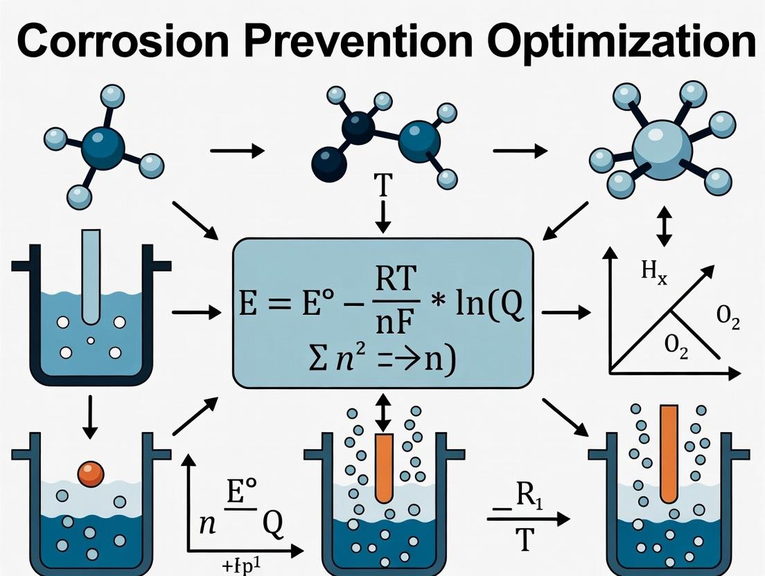
- For corrosion potential (E) prediction related to [Cl⁻], apply the Nernst equation: E = E⁰ - (RT/nF)ln(aCl⁻) where E⁰ is the standard potential for the relevant metal/metal-chloride redox couple.
Visualizations
The Scientist's Toolkit: Research Reagent Solutions
| Item | Function in Experiment |
|---|---|
| Ion-Selective Electrode (ISE) | Sensor with a membrane selective for a specific ion (H⁺, Na⁺, Cl⁻, etc.). Generates a potential proportional to ion activity. |
| Reference Electrode | Provides a stable, constant potential against which the ISE potential is measured (e.g., Ag/AgCl with KCl filling solution). |
| Ionic Strength Adjustor (ISA) | High-concentration inert electrolyte added to all standards and samples to equalize ionic strength, ensuring constant activity coefficients. |
| Standard Solutions | Precise, known concentrations of the target ion used to establish the calibration curve (mV vs. log activity). |
| High-Impedance pH/mV Meter | Measures the high-resistance potential difference between ISE and reference electrode without drawing significant current. |
| Double-Junction Reference Electrode | Prevents contamination of the sample by the reference electrolyte and clogging of the junction, crucial for complex matrices. |
Technical Support Center: Troubleshooting the Nernst Equation in Corrosion Prevention Research
This support center addresses common experimental challenges encountered when applying the Nernst equation (E = E⁰ - (RT/nF) * ln(Q)) to optimize corrosion prevention strategies, particularly in contexts like pharmaceutical equipment biocompatibility and material science.
Frequently Asked Questions (FAQs) & Troubleshooting Guides
Q1: My experimentally measured corrosion potential (E) deviates significantly from the Nernst-predicted value. What are the primary culprits? A: This is a common issue. Follow this systematic checklist:
- Non-Ideal Solution Conditions: The Nernst equation assumes ideal behavior. High ionic strength or specific ion interactions can alter activity coefficients. Use an ionic strength adjuster (ISA) or measure activity directly if possible.
- Liquid Junction Potentials: If your cell uses a salt bridge, unrecognized junction potentials can introduce error. Ensure your reference electrode is appropriate for your solution (e.g., Saturated Calomel Electrode (SCE) for chlorides, Ag/AgCl for non-complexing media).
- Incorrect Reaction Quotient (Q): Verify the chemical species included in your
Qcalculation. For mixed corrosion processes (e.g., involving multiple oxidation states), the dominant couple must be correctly identified. - Slow Kinetics / Non-Equilibrium: The electrode may not be at true electrochemical equilibrium. Allow sufficient stabilization time and confirm open-circuit potential (OCP) stability before measurement.
Q2: How do I accurately determine 'n', the number of electrons transferred, for a complex alloy corrosion process?
A: For pure metals, n is often straightforward. For alloys:
- Potentiodynamic Polarization Analysis: Perform a Tafel plot. The slope of the linear region of the cathodic or anodic branch relates to
n. Use the equationβ = 2.303RT/(αnF), where β is the Tafel slope and α is the charge transfer coefficient (often ~0.5). - Electrochemical Impedance Spectroscopy (EIS): Fit the low-frequency data to a model to estimate charge transfer resistance (Rct), which is inversely related to corrosion current and
n. - Consult Thermodynamic Databases: Use resources like the Pourbaix Atlas to identify the most thermodynamically stable species and their corresponding
nvalues under your experimental pH and potential.
Q3: When monitoring inhibitor efficiency, my calculated corrosion rate from the Nernst/RBE relationship doesn't match mass loss. Why? A: This discrepancy often arises from:
- Localized vs. Uniform Corrosion: The Nernst-derived corrosion current assumes uniform attack. If pitting or crevice corrosion is present, mass loss will be more severe at localized sites than the average current suggests. Complement with surface imaging (SEM).
- Incomplete Redox Couple Capture: Your electrochemical set-up might not be measuring all cathodic reactions (e.g., if oxygen reduction is partially diffusion-controlled).
- Inhibitor Adsorption Dynamics: The inhibitor may form a film that changes the electrochemical mechanism, making the simple Nernst application invalid. Use EIS to model the film resistance and capacitance.
Key Experimental Protocols
Protocol 1: Determining Reversible Potential (E⁰) for a Novel Corrosion-Resistant Alloy
- Prepare Electrolyte: Simulate the operational environment (e.g., phosphate-buffered saline at pH 7.4 for biomaterials).
- Construct Electrochemical Cell: Use a three-electrode system: Alloy as Working Electrode (WE), Pt mesh as Counter Electrode (CE), and Saturated Calomel Electrode (SCE) as Reference.
- Decorate and Stabilize: Polish WE to mirror finish, degrease, and immerse. Monitor OCP until stable (< 2 mV change over 5 min).
- Cyclic Voltammetry (CV): Sweep potential from -0.5V to +1.5V vs. OCP and back at 1 mV/s.
- Analysis: Identify the potential at which the forward and reverse scans intersect on the current-zero line. This is the apparent E⁰ under these conditions. Confirm by varying scan rates.
Protocol 2: Quantifying Inhibitor Efficiency via the Nernst Equation Parameter Shift
- Baseline Measurement: For the uninhibited system, perform linear polarization resistance (LPR) around OCP (±20 mV) to get corrosion current (Icorrbaseline).
- Introduce Inhibitor: Add a known concentration of the corrosion inhibitor (e.g., sodium molybdate) to solution.
- Re-measure & Calculate: After 1 hour of exposure, re-measure OCP and perform LPR to get Icorrinhibited.
- Calculate Efficiency: % Inhibition = [(Icorrbaseline - Icorrinhibited) / Icorrbaseline] * 100.
- Nernst Analysis: The shift in OCP (ΔE) relates to the change in reaction quotient Q due to inhibitor adsorption. Plot ΔE vs. log(inhibitor concentration). A linear region suggests Langmuir-type adsorption.
Table 1: Common Reference Electrodes & Constants for Nernst Calculations
| Electrode | Standard Potential (V vs. SHE at 25°C) | Temperature Coefficient (mV/°C) | Typical Use Case |
|---|---|---|---|
| Standard Hydrogen (SHE) | 0.000 (by definition) | 0.000 | Primary standard |
| Saturated Calomel (SCE) | +0.241 | -0.022 | General aqueous corrosion |
| Silver/Silver Chloride (Ag/AgCl, sat'd KCl) | +0.197 | -0.025 | Biomedical/non-complexing |
| Copper/Copper Sulfate (CSE) | +0.316 | +0.009 | Soil/field corrosion |
Table 2: Impact of Common Experimental Errors on Nernst Potential
| Error Source | Typical Magnitude of Error in E (mV) | Corrective Action |
|---|---|---|
| Temperature fluctuation (±2°C) | ± 0.1 - 0.3 | Use thermostated cell |
| Incorrect ionic strength (10% error in activity) | ± 2.5 | Use ISA or activity meter |
| Junction potential (differing electrolytes) | ± 1 - 30 | Match electrolyte in reference bridge |
| Impurity redox couple (1% conc.) | ± 59 / n | Purify electrolytes, use inert atmosphere |
The Scientist's Toolkit: Research Reagent Solutions
| Item | Function in Corrosion Nernst Experiments |
|---|---|
| Potentiostat/Galvanostat | Applies controlled potential/current to the working electrode and measures the resulting current/potential. Essential for all electrochemical measurements. |
| Luggin Capillary | A probe filled with electrolyte that positions the reference electrode tip close to the WE to minimize solution resistance (iR drop) without shielding. |
| Deaeration Kit (N₂/Ar Sparger) | Removes dissolved oxygen, a common cathodic reactant, to study the anodic metal dissolution reaction in isolation. |
| Ionic Strength Adjuster (ISA - e.g., KNO₃) | Swamps out variable ionic strength between samples, making activity coefficients constant and allowing concentration to be used directly in the Nernst Q. |
| Standardized pH Buffers | Critical for controlling and measuring pH, a key variable in the Nernst equation for reactions involving H⁺ or OH⁻ (e.g., in Pourbaix diagrams). |
| Electrode Polishing Kit (Alumina Slurry) | Provides a reproducible, contaminant-free surface essential for obtaining consistent and accurate equilibrium potentials. |
Visualization: Experimental & Conceptual Diagrams
Technical Support Center: Troubleshooting & FAQs for Electrochemical Corrosion Experiments
Context: This support center provides guidance for experiments within a research thesis focused on optimizing corrosion prevention strategies using the Nernst equation. The following FAQs address common practical issues.
Frequently Asked Questions (FAQs)
Q1: During potentiometric measurement of corrosion potential (E_corr), my readings are unstable and drift significantly. What could be the cause? A: Potential drift is often due to an un-equilibrated system or a contaminated electrode.
- Check 1: Ensure the working electrode (metal sample) is properly polished and cleaned to remove oxides or organic contaminants. Use a standardized polishing protocol (see below).
- Check 2: Allow sufficient time for the open-circuit potential (OCP) to stabilize before recording E_corr. This can take from minutes to several hours depending on the system.
- Check 3: Verify the stability of your reference electrode potential by checking it against a known solution. Ensure there is no clogged junction.
- Protocol - Electrode Polishing: Sequentially polish the metal surface with finer grits of silicon carbide paper (e.g., 600, 800, 1200 grit) under running water to prevent embedding particles. Follow with alumina slurry (1.0 µm and then 0.05 µm) on a polishing cloth. Rinse thoroughly with deionized water and dry.
Q2: When testing an inhibitor, my calculated inhibition efficiency from weight loss and electrochemical methods do not match. Which result should I trust? A: Discrepancies are common as methods measure different aspects of corrosion.
- Cause: Weight loss measures average corrosion rate over the entire test period. Linear Polarization Resistance (LPR) or Tafel extrapolation provide instantaneous electrochemical rates at the time of measurement. Localized corrosion can skew weight loss data.
- Action: Run tests in triplicate. Use electrochemical methods (LPR) for rapid, in-situ screening of inhibitors. Use weight loss as a definitive, long-term validation. Always report both methods with standard deviation.
Q3: My experimental corrosion rate values, derived from the Stern-Geary equation, are orders of magnitude different from literature values for the same metal in a similar environment. A: This typically stems from an incorrect Stern-Geary constant (B).
- Cause: The B-value is not universal. It depends on the specific anodic and cathodic Tafel slopes for your metal/electrolyte/inhibitor system.
- Solution: Perform Tafel extrapolation experiments to determine the actual anodic (βa) and cathodic (βc) Tafel slopes for your system. Calculate B using: B = (βa * βc) / (2.303 * (βa + βc)). Use this calculated B-value in the LPR formula.
Q4: I am trying to apply the Nernst equation to predict the effect of a complexing agent on corrosion potential, but the predicted shift does not match my experiment. Why? A: The standard Nernst equation assumes ideal conditions and specific ion activities.
- Cause 1: You may be using total concentration instead of ion activity. For concentrated or non-ideal solutions, calculate activity using the Debye-Hückel theory.
- Cause 2: The complexing agent may form multiple species with the metal ion (e.g., Fe²⁺, FeL, FeL₂). You must account for the stability constants of all predominant species to calculate the effective concentration of free metal ions [Mⁿ⁺].
- Protocol - Adjusted Nernst Potential Calculation:
- Determine the stability constants (β) for all metal-ligand complexes.
- Calculate the fraction of free metal ion (αM) using speciation software or a manual calculation based on ligand concentration and pH.
- The effective [Mⁿ⁺] = αM * totalmetalconcentration.
- Input this effective concentration into the Nernst equation: E = E⁰ - (RT/nF)ln(αM * [Mtotal]).
Table 1: Typical Stern-Geary Constants (B) for Common Systems
| Metal / System | Assumed B Value (V/decade) | Notes / Conditions |
|---|---|---|
| Mild Steel in acidic solution (active dissolution) | 0.020 - 0.023 | βc for H⁺ reduction dominates. |
| Mild Steel in neutral, aerated solution (oxygen reduction) | 0.052 | Common default value. Should be verified. |
| Copper in neutral water | 0.046 | For mixed charge-transfer control. |
| Aluminum in chloride media | 0.10 - 0.12 | For systems with high βa and βc. |
| Recommendation | Calculate experimentally | Use Tafel extrapolation for accurate results. |
Table 2: Comparison of Corrosion Rate Measurement Techniques
| Method | Measures | Time Required | Pros | Cons |
|---|---|---|---|---|
| Weight Loss | Average mass loss | Days to weeks | Direct, simple, definitive. | Slow, no mechanistic insight. |
| Tafel Extrapolation | Instantaneous rate, βa, βc | Minutes to hours | Provides kinetic parameters. | Can disturb the system; requires expert fitting. |
| Linear Polarization (LPR) | Instantaneous polarization resistance (Rp) | Minutes | Non-destructive, fast, in-situ. | Requires accurate B-value. |
| Electrochemical Impedance Spectroscopy (EIS) | Rp, solution resistance, capacitance | 30 mins to hours | Models interface processes, non-destructive. | Complex data analysis. |
The Scientist's Toolkit: Research Reagent Solutions
Table 3: Essential Materials for Electrochemical Corrosion Studies
| Item | Function | Example & Notes |
|---|---|---|
| Potentiostat/Galvanostat | Applies controlled potential/current and measures electrochemical response. | Instruments from Gamry, BioLogic, Metrohm. Key for all electrochemical methods. |
| 3-Electrode Cell Kit | Provides a stable experimental setup. | Includes working (metal sample), reference (e.g., Saturated Calomel - SCE), and counter (e.g., Pt mesh) electrodes. |
| Ag/AgCl Reference Electrode | Stable, reproducible reference potential. | Commonly used. Fill with appropriate KCl solution (3M or saturated). |
| Corrosive Electrolyte | Simulates the environment of interest. | 0.1M HCl for acidic corrosion, 3.5% NaCl for simulating seawater. |
| Corrosion Inhibitor | Compound under test for prevention. | e.g., Sodium phosphate, Benzotriazole (BTAH) for copper, proprietary organic compounds. |
| Polishing Supplies | Creates a reproducible, clean metal surface. | Silicon carbide papers (various grits), alumina powder (0.05µm), polishing cloths. |
| Deaeration System | Removes oxygen to study specific mechanisms. | Sparging with high-purity nitrogen or argon gas for 20+ minutes prior to and during experiment. |
| Faraday Cage | Shields the electrochemical cell from external electromagnetic noise. | Essential for low-current (nA-µA) measurements like for coated samples. |
Experimental Protocols & Visualizations
Protocol: Standard Three-Electrode Setup for Corrosion Potential Monitoring
- Preparation: Polish the working electrode (WE) as per the protocol in FAQ A1. Clean the counter electrode (CE) with acid and flame. Check reference electrode (RE) filling solution.
- Assembly: Place the WE, RE, and CE in the electrochemical cell containing the electrolyte. Ensure the RE's Luggin capillary is positioned close (~2 mm) to the WE surface.
- Connection: Connect the electrodes to the potentiostat: green (WE), red (CE), white (RE). Place the cell in a Faraday cage.
- Initialization: In the potentiostat software, select the "Open Circuit Potential" (OCP) experiment. Set the duration to a minimum of 1 hour or until the potential stabilizes (±2 mV over 5 minutes).
- Recording: Start the experiment. The stabilized potential value is recorded as E_corr (corrosion potential).
Title: Workflow for Measuring Corrosion Potential (E_corr)
Title: Nernst Equation Role in Corrosion Research
Technical Support Center
Troubleshooting Guides & FAQs
Q1: Our potentiometric pH sensor shows a drifting, non-Nernstian response during long-term cell culture monitoring. What could be the cause and solution? A: Drift is often caused by reference electrode contamination or clogging of the pH-sensitive glass membrane. Proteins and cellular debris can foul the surface.
- Troubleshooting Steps:
- Calibration Check: Perform a fresh two-point calibration (pH 4.01 & 7.00 buffers). If slope is not between -54 mV/pH to -60 mV/pH (at 37°C), the sensor is impaired.
- Inspection: Visually check for coating or particles on the sensor bulb.
- Cleaning Protocol: Gently rinse with deionized water. If fouling persists, immerse the sensing bulb in a 0.1M HCl solution for 5-10 minutes, followed by a 30-minute soak in saturated KCl. Rinse thoroughly and recalibrate.
- Reference Junction Maintenance: For Ag/AgCl references, ensure the porous junction is kept hydrated. Store in 3M KCl solution when not in use.
Q2: Chloride ion-selective electrode (ISE) measurements in biological fluids (e.g., serum) yield consistently low values. How do we correct for this? A: This is a classic interference issue. Proteins and bicarbonate in biological samples can complex Cl⁻ or alter ionic strength, affecting the Nernstian potential.
- Troubleshooting Steps:
- Sample Preparation: Dilute the sample 1:10 with a high-ionic-strength background electrolyte (e.g., 5M NaNO₃). This minimizes the "ionic strength mismatch" between samples and standards and reduces protein interference.
- Standard Addition Method: Use the method of standard additions to the biological sample directly. This accounts for matrix effects.
- Calibration Match: Prepare calibration standards in a matrix that mimics your sample (e.g., a synthetic serum background). Do not calibrate with pure NaCl solutions.
Q3: The dissolved oxygen (DO) amperometric sensor signal is unstable and noisy in a bioreactor, affecting our corrosion potential (E_corr) measurements. A: Noise often stems from electrical interference or flow sensitivity. Fluctuating O₂ consumption by cells can also cause real signal variation.
- Troubleshooting Steps:
- Electrical Grounding: Ensure the bioreactor, sensor, and potentiostat are properly grounded to a common point. Use shielded cables.
- Stirring/Flow Rate: Maintain a constant, controlled stir rate. Amperometric DO sensors are flow-sensitive. Mark a standard stirring setting for reproducible measurements.
- Membrane Integrity: Check the sensor's Teflon/FEP membrane for tears or bubbles. Replace if damaged. Ensure electrolyte is present in Clark-type sensors.
- Protocol for Correlation: When measuring E_corr, log DO and potential simultaneously with a high sampling rate (e.g., 1 Hz) to identify true correlations versus artifact.
Q4: How do we validate that our potentiometric system is obeying the Nernst equation for a specific ion (like H⁺ or Cl⁻) in a complex biomedical medium? A: Perform a Nernstian slope recovery experiment.
- Experimental Protocol:
- Prepare a base matrix that mimics your test medium (e.g., PBS, cell culture media without serum).
- Spike this base matrix with known, increasing concentrations of your target ion. For pH, use small volumes of strong acid/base. For Cl⁻, use a concentrated NaCl solution.
- Measure the potential (mV) at each concentration.
- Plot E (mV) vs. log10(ion activity). The slope should be close to the theoretical Nernst slope (59.16 mV/decade at 25°C for monovalent ions; ~61.5 mV/decade at 37°C).
- A deviation >±5% indicates significant matrix interference requiring the sample preparation methods noted in Q2.
Table 1: Critical Nernstian Parameters for Biomedical Sensing
| Parameter | Typical Sensor Type | Theoretical Nernst Slope (at 37°C) | Key Interferences in Biomedical Samples | Optimal Calibration Matrix |
|---|---|---|---|---|
| pH | Potentiometric (Glass Membrane) | -61.54 mV/pH | Na⁺ (at high pH, "alkaline error"), Proteins (fouling) | Standard pH buffers (4.01, 7.00, 10.01) |
| Chloride (Cl⁻) | Potentiometric (ISE Crystal/Liquid Membrane) | +61.54 mV/decade | SCN⁻, I⁻, Br⁻, OH⁻, Bicarbonate, Proteins | Ionic Strength Adjusted (ISA) Standards |
| Dissolved Oxygen | Amperometric (Clark Electrode) | -- (Current is proportional to pO₂) | H₂S, SO₂, Cl₂ (react with cathode), Stirring Rate | Air-saturated water (100%), Na₂SO₃ solution (0%) |
The Scientist's Toolkit
Table 2: Essential Research Reagent Solutions for Nernstian Parameter Experiments
| Item | Function in Experiment |
|---|---|
| Ionic Strength Adjuster (ISA) for Cl⁻ | Contains high concentration of inert electrolyte (e.g., NaNO₃) to fix ionic strength across samples and standards, minimizing junction potential errors. |
| Saturated KCl (for Reference Electrodes) | Maintains a stable and reproducible liquid junction potential for Ag/AgCl reference electrodes. Must be used for storage and refilling. |
| pH Buffer Solutions (NIST Traceable) | Provides known, stable activity of H⁺ ions for accurate calibration of pH sensors across the physiological range (pH 4-10). |
| Zero Oxygen Solution (1M Na₂SO₃) | Chemically removes oxygen to establish a reliable 0% DO baseline for amperometric sensor calibration. |
| Synthetic Interstitial Fluid or PBS | Provides a physiologically relevant, protein-free matrix for preparing calibration standards to better match sample background. |
| Electrode Cleaning Solution (0.1M HCl / Pepsin) | Gently removes proteinaceous biofouling from pH and ISE membranes without damaging the sensitive surface. |
Experimental Workflow & Relationship Diagrams
Establishing the Equilibrium Potential for Critical Half-Cells (Fe/Fe2+, Cr/Cr3+, etc.)
Technical Support Center
Troubleshooting Guides & FAQs
Q1: During potentiometric measurement of the Fe/Fe2+ half-cell, the voltage reading is unstable and drifts continuously. What could be the cause? A: This is typically due to oxygen contamination or an improperly prepared electrode surface. Ensure the electrolyte is thoroughly deaerated by bubbling with an inert gas (e.g., nitrogen or argon) for at least 30 minutes prior to measurement. Re-prepare the iron electrode by sequentially polishing with finer grits of alumina (down to 0.05 µm), rinsing with deionized water, and quickly transferring to the deaerated solution.
Q2: The calculated equilibrium potential for my Cr/Cr3+ cell deviates significantly from the standard literature value. How should I troubleshoot? A: First, verify the activity/concentration of Cr3+ ions. Use an analytical technique like ICP-MS to confirm the exact concentration. Then, check for the presence of complexing agents or impurities in your solution that may alter ion activity. Ensure the pH is controlled, as hydrolysis of Cr3+ can form species like Cr(OH)2+, affecting the potential. Recalculate using the Nernst equation with the verified activity.
Q3: My corrosion potential measurements for a dual half-cell setup are not reproducible between experimental runs. A: Standardize your experimental protocol. Key factors include: 1) Electrode History: Use a fresh electrode surface for each run or document and replicate the pre-treatment exactly. 2) Solution Purity: Use high-purity reagents (e.g., TraceSELECT) and document water resistivity (>18 MΩ·cm). 3) Equilibrium Criteria: Define a strict criterion for equilibrium (e.g., potential change < 0.1 mV/min for 10 minutes) and apply it consistently.
Q4: How do I properly account for liquid junction potentials when measuring half-cell potentials against a reference electrode? A: Liquid junction potentials (Ej) are a common source of error. To minimize: 1) Use a salt bridge with a high concentration of an electrolyte with nearly equal cation and anion mobility (e.g., saturated KCl for calomel electrodes). 2) For precise work, measure the potential with and without a salt bridge ionic strength adjuster. 3) The Ej can be estimated using the Henderson equation and should be reported as a potential uncertainty in your thesis methodology.
Table 1: Standard Reduction Potentials (E°) and Key Parameters at 298.15 K
| Half-Cell Reaction | Standard Potential, E° (V vs. SHE) | Temperature Coefficient (∂E°/∂T) mV/K | Key Experimental Consideration |
|---|---|---|---|
| Fe²⁺ + 2e⁻ ⇌ Fe(s) | -0.44 | -0.05 | Extreme O₂ sensitivity; requires inert atmosphere. |
| Cr³⁺ + 3e⁻ ⇌ Cr(s) | -0.74 | ~0.10 | Slow kinetics; long equilibrium time required. |
| Zn²⁺ + 2e⁻ ⇌ Zn(s) | -0.76 | -0.10 | Reliable and reproducible system for calibration. |
| Cu²⁺ + 2e⁻ ⇌ Cu(s) | +0.34 | +0.01 | Stable, often used as a secondary reference. |
Table 2: Common Experimental Issues and Solutions
| Symptom | Likely Cause | Corrective Action |
|---|---|---|
| Noisy Potential Signal | Electrical interference, poor connections. | Use shielded cables, Faraday cage, check all contacts. |
| Potential Drift Over Hours | Changing ion concentration (e.g., from corrosion), temperature drift. | Use larger solution volume, implement temperature control (±0.1°C). |
| Inconsistent Readings Between Cells | Uncalibrated reference electrode, contaminated salt bridge. | Calibrate reference vs. known standard (e.g., Zn/Zn²⁺), replace bridge electrolyte. |
Experimental Protocol: Determining Fe/Fe²⁺ Equilibrium Potential
Objective: To accurately measure the equilibrium potential of the Fe/Fe²⁺ half-cell for use in corrosion thermodynamics modeling.
Materials: See "Research Reagent Solutions" below.
Procedure:
- Electrode Preparation: Polish a high-purity (99.99%) iron rod (5 mm diameter) with alumina slurry (1.0, 0.3, and 0.05 µm sequentially). Sonicate in ethanol for 5 minutes, then in deionized water. Dry under a stream of N₂.
- Electrolyte Preparation: Prepare 0.01 M FeSO₄ solution in 0.1 M NaCl as supporting electrolyte. Adjust pH to 3.0 using deaerated HCl to prevent Fe²⁺ oxidation and hydroxide precipitation.
- Deaeration: Transfer solution to the electrochemical cell. Sparge vigorously with high-purity argon for 30 minutes. Maintain a positive pressure of argon above the solution throughout the experiment.
- Cell Assembly: Under argon flow, insert the prepared Fe working electrode, a salt bridge (filled with 0.1 M NaCl) connected to a saturated calomel reference electrode (SCE), and a platinum wire counter electrode.
- Measurement: Allow the system to equilibrate. Monitor the open-circuit potential (OCP) vs. time. Record the potential when the change is less than 0.05 mV per minute for 15 consecutive minutes. This is the equilibrium potential (E_eq).
- Data Correction: Correct the measured potential to the Standard Hydrogen Electrode (SHE) scale using: E (vs. SHE) = E (vs. SCE) + 0.241 V. Apply the Nernst equation: Eeq = E° - (RT/2F) * ln(aFe²⁺) to validate, where a_Fe²⁺ is the estimated activity.
Research Reagent Solutions
| Item | Function in Experiment |
|---|---|
| High-Purity Iron Electrode (99.99%) | Provides a defined, low-impurity surface for the Fe/Fe²⁺ redox reaction. |
| FeSO₄·7H₂O (TraceSELECT grade) | Source of Fe²⁺ ions with minimal metallic impurities that could plate and contaminate the electrode. |
| NaCl (Suprapur grade) | Provides inert supporting electrolyte to control ionic strength and minimize junction potentials. |
| Deoxygenated HCl (prepared under Ar) | For pH adjustment without introducing oxidizing agents. |
| Alumina Polishing Suspension (0.05 µm) | Creates a reproducible, clean, and smooth electrode surface. |
| Argon Gas (Ultra High Purity, O₂ < 1 ppm) | Removes dissolved oxygen to prevent oxidation of Fe²⁺ to Fe³⁺. |
| Saturated Calomel Electrode (SCE) | Stable, commercial reference electrode with a well-defined potential. |
Diagrams
Diagram 1: Experimental Workflow for Half-Cell Potential Measurement
Diagram 2: Nernst Equation Logic in Corrosion Prevention Thesis
From Theory to Bench: A Step-by-Step Guide to Nernst-Driven Corrosion Prediction
Technical Support Center: Troubleshooting & FAQs
Frequently Asked Questions
Q1: My measured open-circuit potential (OCP) is highly unstable and never reaches a steady state. What could be the cause? A: This is often due to an insufficiently equilibrated system or a contaminated electrolyte. First, ensure your simulated physiological fluid (e.g., PBS, Hank's solution) has been freshly prepared, deaerated with nitrogen or argon for at least 30 minutes, and allowed to thermally equilibrate in the cell for 1 hour before immersion. Clean the working electrode (the metal sample) rigorously via a standard protocol of grinding, polishing, and ultrasonic cleaning in ethanol and distilled water. Ensure the reference electrode (e.g., Saturated Calomel Electrode - SCE) is filled and functioning correctly.
Q2: How do I validate my reference electrode's potential in my specific simulated fluid? A: Perform a calibration check using a known redox couple. A common method is to measure the potential of a clean Platinum wire in the same fluid equilibrated with air, against your reference electrode. The potential for the Oxygen Reduction Reaction (ORR) in aerated neutral solutions should be approximately +0.2 to +0.3 V vs. SCE. A significant deviation (>50 mV) suggests reference electrode contamination or junction failure.
Q3: When calculating the theoretical corrosion potential (E_corr) using the mixed potential theory and Nernst equation, my calculated value deviates significantly from the experimental value. Why? A: Theoretical calculations assume ideal, pure metals and simple redox couples (e.g., Fe/Fe2+, O2/H2O). Real systems in physiological fluids are complex. The deviation can be due to: 1) Formation of complex ions (e.g., FeCl+, Fe(HPO4)2-) which alter ion activity, 2) The presence of organic molecules (e.g., proteins, amino acids) that adsorb and inhibit/anodize reactions, 3) The formation of a non-equilibrium passive film not accounted for in the simple Nernst equation. Use the theoretical value as a baseline and analyze the deviation to gain insights into these complex interactions.
Q4: My potentiodynamic polarization curve shows no clear Tafel region for accurate corrosion current (Icorr) extraction. How should I proceed? A: This is common for metals that passivate quickly (e.g., stainless steels, titanium alloys) in physiological fluids. Do not force a Tafel fit. Instead, report the corrosion potential (Ecorr) from the intersection of anodic and cathodic slopes, even if linear, and note the low current density in the passive region. Consider using Electrochemical Impedance Spectroscopy (EIS) to calculate polarization resistance (Rp) and derive I_corr using the Stern-Geary equation, which is more reliable for such systems.
Key Experimental Protocols
Protocol 1: Standard Three-Electrode Cell Setup for OCP Measurement
- Electrolyte Preparation: Prepare 1 liter of Phosphate Buffered Saline (PBS, pH 7.4) using reagent-grade salts and ultrapure water (18.2 MΩ·cm). Deaerate with high-purity N2 gas for 45 minutes prior to use and maintain a blanket during measurement.
- Working Electrode (WE) Preparation: Cut the test alloy into 1 cm² coupons. Sequentially wet-polish with SiC paper from 400 to 2000 grit. Rinse with distilled water, then ultrasonically clean in acetone for 5 minutes, followed by ethanol for 5 minutes. Air-dry in a laminar flow hood.
- Cell Assembly: Place the electrolyte in a double-jacketed glass cell connected to a 37°C circulator. Insert the WE, a Platinum mesh counter electrode (CE), and the reference electrode (RE). Ensure the RE's Luggin capillary tip is approximately 2 mm from the WE surface.
- Data Acquisition: Connect the electrodes to the potentiostat. Measure the OCP for a minimum of 3600 seconds (1 hour) or until the potential change is less than 1 mV over 300 seconds. Record the final stable potential as E_ocp.
Protocol 2: Potentiodynamic Polarization for Corrosion Parameter Extraction
- Initialization: After Protocol 1 (OCP measurement), begin the polarization scan from -0.25 V vs. OCP to +0.8 V vs. OCP.
- Scan Parameters: Set a scan rate of 0.167 mV/s (1 mV/min). This slow rate is critical for quasi-equilibrium conditions in low-conductivity physiological fluids.
- Data Analysis: Plot potential (E) vs. log |current density| (log |i|). Identify the linear regions (±50-100 mV from Ecorr) on the anodic and cathodic branches. Extrapolate these Tafel regions to their intersection. The intersection point's x-coordinate is log(Icorr) and its y-coordinate is E_corr.
Table 1: Calculated and Measured Corrosion Potentials for Pure Metals in Deaerated PBS (pH 7.4) at 37°C
| Metal (Redox Couple) | Nernst Calculated E (V vs. SHE) | Converted E (V vs. SCE) | Typical Experimental E_corr (V vs. SCE) | Notes |
|---|---|---|---|---|
| Iron (Fe/Fe²⁺) | -0.64 | -0.88 | -0.65 ± 0.10 | Deviation due to Fe(OH)₂/Fe₂O₃ film formation. |
| Zinc (Zn/Zn²⁺) | -0.86 | -1.10 | -1.05 ± 0.05 | Good agreement; minimal passivation in Cl⁻ media. |
| Magnesium (Mg/Mg²⁺) | -2.37 | -2.61 | -1.65 ± 0.15 | Large deviation due to high negative difference effect and H₂ evolution. |
| Oxygen Reduction (O₂/H₂O) | +0.81 | +0.57 | +0.20 to +0.30 | Mixed potential controlled by diffusion-limited O₂, not equilibrium. |
Note: SHE = Standard Hydrogen Electrode; SCE = Saturated Calomel Electrode (E = +0.241 V vs. SHE). Calculated using Nernst equation: E = E⁰ - (0.0591/n)log(Q) at 37°C, with assumed ion activity of 10⁻⁶ M.*
The Scientist's Toolkit
Table 2: Essential Research Reagent Solutions for Corrosion Experiments
| Item | Function & Specification |
|---|---|
| Phosphate Buffered Saline (PBS) | Standard simulated interstitial fluid. Provides chloride ions for pitting and phosphates for possible precipitation. Use pH 7.4. |
| Hank's Balanced Salt Solution (HBSS) | More complex physiological simulant containing essential inorganic ions (Ca²⁺, Mg²⁺, HCO₃⁻) for studying biomaterial degradation. |
| Ringer's Solution | Simulates body fluid ionics; essential for testing implants where carbonate/bicarbonate buffering is relevant. |
| 0.9 wt% NaCl (Saline) | Basic chloride environment for studying uniform corrosion and pitting susceptibility. |
| High-Purity Nitrogen/Argon Gas | For deaeration to study corrosion mechanisms without dissolved O₂, isolating anodic metal dissolution. |
| Potentiostat/Galvanostat | Core instrument for applying controlled potentials/currents and measuring electrochemical response. Requires Faraday cage for low-current measurements. |
| Ag/AgCl (in saturated KCl) Reference Electrode | Common, stable reference electrode. Preferred over SCE for 37°C work due to lower temperature coefficient. |
| Luggin Capillary | A salt-bridge extension from the RE to minimize iR drop and isolate the RE from the test solution. |
Experimental & Conceptual Diagrams
Title: Workflow for Theoretical vs. Experimental E_corr Analysis
Title: Three-Electrode Cell Schematic for Corrosion Testing
Title: From Nernst Equation to Theoretical E_corr
Technical Support Center: Troubleshooting & FAQs
Q1: During experimental validation of a calculated Pourbaix diagram for a novel alloy, the measured potential in my electrochemical cell is unstable and drifts significantly over time. What could be the cause and how do I fix it?
A: Unstable potential readings are commonly due to reference electrode issues or insufficient electrolyte conditioning.
- Primary Cause: A clogged or contaminated reference electrode (e.g., Saturated Calomel Electrode - SCE, Ag/AgCl) junction.
- Troubleshooting Protocol:
- Verify Reference Electrode: Check the filling solution level and ensure the porous frit is not clogged. Soak in fresh KCl solution (saturated for SCE, 3M for Ag/AgCl) for 30 minutes.
- Check Electrical Connections: Ensure all cables are secure and the working electrode is properly isolated.
- Purge Electrolyte: De-aerate the electrolyte solution with an inert gas (e.g., N₂, Ar) for at least 20 minutes prior to and during measurement to remove dissolved oxygen, which can cause competing redox reactions.
- Condition the Working Electrode: Perform a pre-experiment cyclic voltammetry scan to stabilize the electrode surface before potentiostatic measurements.
Q2: My experimentally determined stability zone for a metallic implant material is much narrower than the zone predicted by the Nernst equation, especially in the neutral pH region. Why does this discrepancy occur?
A: This is a frequent issue when theoretical Pourbaix diagrams are applied to real biomedical environments. The diagram predicts thermodynamic stability, while experiments reveal kinetic limitations and complex speciation.
- Primary Cause: The theoretical calculation assumes only simple aquo-ions (e.g., Fe²⁺, Fe³⁺), but in physiological solutions, complexation with anions (Cl⁻, HPO₄²⁻, citrate) and organic molecules (proteins) stabilizes soluble species, enlarging the corrosion domain.
- Troubleshooting Protocol:
- Recalculate with Correct Species: Use thermodynamic software (e.g., Hydra/Medusa, FactSage) to recalculate the diagram, including relevant ligand concentrations (e.g., 0.15 M Cl⁻, 1-10 mM phosphate).
- Experimental Verification: Conduct Potentiodynamic Polarization experiments in simulated body fluid (SBF) and compare the corrosion potential (E_corr) and passivation behavior to the adjusted diagram.
- Surface Analysis: Post-experiment, use X-ray Photoelectron Spectroscopy (XPS) to identify the actual surface film composition, which may be a mixed oxide/hydroxide or incorporate anions.
Q3: When attempting to map the "immunity" zone of a drug container material, how do I accurately set and control the pH and potential in a borate buffer system?
A: Precise control is achieved using a three-electrode potentiostat setup with a pH-stat.
- Experimental Protocol:
- Setup: Use a glass electrochemical cell with a working electrode (your material), a Pt mesh counter electrode, and a sealed, double-junction reference electrode (to avoid KCl contamination).
- Potential Control: Connect the cell to a potentiostat. Set the desired potential (vs. REF) based on your calculated Pourbaix diagram. The potentiostat will maintain this potential by adjusting current between the working and counter electrodes.
- pH Control: Use an automated pH-stat system. The pH electrode feeds data to a controller, which dispenses small volumes of dilute NaOH or H₃BO₃/HCl to maintain the target pH within ±0.02 units.
- Validation: Periodically measure the open-circuit potential (OCP) and pH independently with a calibrated meter to confirm system stability.
Q4: For my corrosion prevention thesis, I need to integrate kinetic data (corrosion rates) with the thermodynamic Pourbaix map. What is the best experimental workflow to overlay these datasets?
A: The workflow combines Electrochemical Impedance Spectroscopy (EIS) and Potentiodynamic Polarization with Pourbaix mapping.
Diagram Title: Workflow for Kinetic-Thermodynamic Pourbaix Integration
Table 1: Common Reference Electrodes for Pourbaix Experiments
| Electrode | Potential vs. SHE (25°C) | Typical Use Case | Stability Consideration |
|---|---|---|---|
| Standard Hydrogen (SHE) | 0.000 V (by definition) | Primary standard, theoretical | Requires H₂ gas, lab use only |
| Saturated Calomel (SCE) | +0.241 V | General aqueous electrochemistry | Temperature sensitive, KCl leakage |
| Ag/AgCl (sat. KCl) | +0.197 V | Biomedical/buffer solutions | Stable, easy miniaturization |
| Ag/AgCl (3M KCl) | +0.210 V | High chloride media | Less temperature sensitive than SCE |
| Hg/HgO (1M NaOH) | +0.140 V | Strong alkaline media | For high-pH studies only |
Table 2: Impact of Anions on Measured Corrosion Potential (E_corr) of 316L Steel (pH 7.4)
| Anion (0.1M) | Complexing Agent? | Average E_corr shift vs. Pure Water | Observed Effect on Passivation |
|---|---|---|---|
| Chloride (Cl⁻) | Weak | -85 mV | Localized breakdown (pitting) |
| Citrate (C₆H₅O₇³⁻) | Strong | -210 mV | Complete dissolution, no passivation |
| Phosphate (HPO₄²⁻) | Moderate | +50 mV | Stabilizes passive film |
| Bicarbonate (HCO₃⁻) | Weak | -25 mV | Slight inhibition |
The Scientist's Toolkit: Key Research Reagent Solutions
Table 3: Essential Materials for Experimental Pourbaix Diagram Mapping
| Item | Function / Composition | Critical Role in Experiment |
|---|---|---|
| Potentiostat/Galvanostat | e.g., Biologic SP-150, Ganny Interface 1010E | Applies and precisely controls electrode potential for Nernstian measurements. |
| Double-Junction Reference Electrode | Inner: Ag/AgCl; Outer: KNO₃ or sample electrolyte | Provides stable reference potential while preventing contamination of test solution. |
| pH-Stat System | pH meter, controller, burette with titrant (acid/base) | Maintains constant pH for hours/days, essential for mapping vertical (pH-dependent) boundaries. |
| De-aerated Electrolyte | e.g., 0.1M Na₂SO₄, purged with Argon (Ar) >30 min. | Removes O₂, which acts as an unwanted oxidant, simplifying the redox system to M/Mⁿ⁺/MxOy. |
| Simulated Body Fluid (SBF) | Kokubo's recipe: contains Cl⁻, HCO₃⁻, HPO₄²⁻, etc. | For biomedical alloy studies, provides realistic anion complexation not in simple aqueous diagrams. |
| Thermodynamic Software | Hydra/Medusa, FactSage, OLI Analyzer | Calculates theoretical Pourbaix diagrams including complex soluble species beyond simple ions. |
Technical Support Center
FAQs & Troubleshooting Guides
Q1: My potentiostat measurement for galvanic current (I_galv) between coupled alloys is unstable and noisy. What could be the cause? A: This is commonly caused by a poor reference electrode connection or an unstable open circuit potential (OCP) prior to coupling. Ensure your reference electrode (e.g., Saturated Calomel Electrode) is properly filled and placed within the Luggin capillary. Follow this protocol: 1) Measure and log OCP for each isolated electrode for at least 1 hour until stable (< ±2 mV/min drift). 2) Ensure all connections are clean and secure. 3) Perform the coupling experiment in a Faraday cage if electrical noise from other lab equipment is suspected.
Q2: How do I accurately calculate the theoretical galvanic corrosion risk using the Nernst equation before an experiment? A: Use the Nernst equation to predict the corrosion potential (Ecorr) for each alloy separately: E = E° - (RT/nF) ln(Q), where Q is the reaction quotient for the metal dissolution. The alloy with the more noble Ecorr will act as the cathode. The driving force is the potential difference (ΔE). However, this is a thermodynamic prediction; kinetics (polarization resistance) control the actual corrosion rate. You must supplement with experimental polarization data.
Q3: My simulated body fluid (SBF) electrolyte composition is precipitating. How does this affect my corrosion measurements? A: Precipitation alters the ionic concentration, changing the solution's conductivity and the effective area of the working electrode. This invalidates assumptions for the Stern-Geary equation used to calculate corrosion current density. To prevent this: 1) Prepare SBF at a lower temperature (e.g., 5°C). 2) Add the reagents in the exact order specified in Kokubo's protocol. 3) Continuously stir and maintain the solution at 36.5°C ± 0.5, and do not use it beyond 48 hours after preparation.
Q4: How do I determine the effective cathode-to-anode surface area ratio (Ac/Aa) in a complex multi-alloy device? A: This requires a combination of physical measurement and electrochemical modeling. Protocol: 1) Use 3D scanning or precise CAD models of the device to determine the physical surface area of each component. 2) In your potentiostat setup, use a zero-resistance ammeter (ZRA) mode to measure the galvanic current between specific paired alloys. 3) Perform potentiodynamic polarization on each alloy separately to obtain Tafel slopes. 4) Use the mixed-potential theory and the measured I_galv to back-calculate the electrochemically active area ratio, which may differ from the physical ratio due to passivation.
Q5: When testing in a multi-electrode array (MEA), how do I isolate the signal from two specific alloys when many are connected? A: Modern MEA systems use multiplexing. Ensure your experimental workflow includes a baseline scan: 1) Measure OCP for all electrodes. 2. Program the sequence to couple only two electrodes at a time via the multiplexer, recording current between each specific pair. 3. Use a common reference electrode for all potential measurements. Data is typically processed using software to generate a current and potential map for each coupling combination.
Data Presentation
Table 1: Standard Reduction Potentials (E°) & Typical Corrosion Potentials in SBF (vs. SCE)
| Alloy/Metal | E° (V, vs. SHE) | Typical E_corr in SBF (V, vs. SCE) | Common Role in Galvanic Couple |
|---|---|---|---|
| Magnesium (Mg) | -2.37 | -1.60 to -1.50 | Anode (Sacrificial) |
| Zinc (Zn) | -0.76 | -1.05 to -0.95 | Anode |
| Iron (Fe) | -0.44 | -0.70 to -0.50 | Anode/Cathode |
| 316L Stainless Steel | -0.43* | -0.20 to +0.10 | Cathode |
| Cobalt-Chrome (CoCr) | -0.28* | -0.15 to +0.15 | Cathode |
| Titanium (Ti) | -1.63 | -0.10 to +0.20 | Cathode (Passive) |
| Platinum (Pt) | +1.18 | +0.20 to +0.50 | Cathode (Inert) |
*Approximate for base metal.
Table 2: Key Electrochemical Parameters for Corrosion Rate Calculation
| Parameter | Symbol | Unit | Typical Measurement Method | Relevance to Galvanic Corrosion |
|---|---|---|---|---|
| Corrosion Potential | E_corr | V (vs. Ref.) | Open Circuit Potential (OCP) | Predicts which alloy corrodes. |
| Corrosion Current Density | i_corr | A/cm² | Tafel Extrapolation / EIS (Stern-Geary) | Base corrosion rate without coupling. |
| Anodic Tafel Slope | β_a | V/decade | Potentiodynamic Polarization | Kinetics of metal dissolution. |
| Cathodic Tafel Slope | β_c | V/decade | Potentiodynamic Polarization | Kinetics of reduction reaction (e.g., O₂). |
| Polarization Resistance | R_p | Ω·cm² | Linear Polarization / EIS | Inversely proportional to i_corr. |
| Galvanic Current | I_galv | A | Zero-Resistance Ammetry (ZRA) | Direct measure of coupled corrosion rate. |
Experimental Protocols
Protocol 1: Baseline Potentiodynamic Polarization for Single Alloy Objective: Obtain Tafel constants (βa, βc) and corrosion current density (i_corr) for an alloy. Method:
- Setup: Use a standard three-electrode cell: Working Electrode (alloy sample, 1 cm² exposed), Counter Electrode (Pt mesh), Reference Electrode (Saturated Calomel Electrode, SCE).
- Stabilization: Immerse sample in electrolyte (e.g., SBF, PBS) and monitor OCP for 1 hour or until stable (< ±1 mV/min).
- Polarization: Scan potential from -0.25 V to +0.25 V relative to E_corr at a slow scan rate (0.166 mV/s).
- Analysis: Use software to perform Tafel extrapolation on the linear regions (±50-100 mV from Ecorr) of the anodic and cathodic branches to determine βa, βc, and icorr.
Protocol 2: Zero-Resistance Ammetry (ZRA) for Galvanic Couple Objective: Measure the galvanic current flowing between two dissimilar alloys when electrically shorted. Method:
- Setup: Two identical-sized samples (e.g., 1 cm² each) of Alloy A and Alloy B as working electrodes. Connect both to the ZRA channel of the potentiostat. Include a common reference electrode.
- Pre-measurement: Measure and record individual OCPs for 30 minutes.
- Coupling: Initiate ZRA measurement, electrically shorting the two working electrodes through the instrument. Record Igalv and the coupled potential (Egalv) for 24 hours.
- Post-analysis: Relate I_galv to the corrosion rate of the anodic member using Faraday's law.
Protocol 3: Multi-Electrode Array (MEA) Screening Objective: Rapidly assess galvanic interactions between multiple alloys in one set-up. Method:
- Array Fabrication: Miniature electrodes (wires, ~1 mm²) of each alloy of interest are embedded in an inert epoxy, polished to a uniform surface.
- Configuration: Each electrode is connected to an independent channel of an MEA system. A common reference and counter electrode are used.
- Automated Scanning: Software sequentially couples every possible pair of electrodes in a ZRA-like mode, measuring Igalv and Egalv for each pair for a set duration (e.g., 10 min/pair).
- Data Mapping: Results are compiled into a matrix to identify high-risk couples.
Visualizations
Title: Experimental Workflow for Galvanic Risk Assessment
Title: Multi-Electrode Array (MEA) Setup Diagram
The Scientist's Toolkit
Table 3: Key Research Reagent Solutions & Materials
| Item | Function | Critical Specification/Note |
|---|---|---|
| Potentiostat/Galvanostat with ZRA | Applies potential/current and measures electrochemical response. | Must have Zero-Resistance Ammetry (ZRA) mode for galvanic coupling studies. |
| Simulated Body Fluid (SBF) | In-vitro electrolyte mimicking ionic composition of blood plasma. | Prepare per Kokubo protocol (Tris-buffered, pH 7.40 at 36.5°C) to ensure reproducibility. |
| Saturated Calomel Electrode (SCE) | Stable reference electrode for potential measurement. | Maintain saturated KCl solution level; check for clogged frit. |
| Luggin Capillary | Places reference electrode close to working electrode without shielding. | Minimizes solution resistance (iR drop) in high-resistivity electrolytes. |
| Electrode Mounting Epoxy | Insulates all but a defined surface area of the sample. | Use chemically inert epoxy (e.g., epoxy resin) to prevent crevice corrosion. |
| Non-conductive Sample Holder | Holds working electrode in place. | Materials like Teflon or Nylon are ideal to avoid stray currents. |
| Faraday Cage | Electrically shielded enclosure for the cell. | Eliminates external noise for sensitive current measurements (e.g., nA level). |
| Standard Polishing Supplies | Creates a reproducible, contaminant-free surface. | SiC paper (up to 2000 grit), alumina slurry (0.05 µm), ultrasonic cleaner. |
Technical Support & Troubleshooting Center
Frequently Asked Questions (FAQs)
Q1: My measured open circuit potential (OCP) for 316L stainless steel in PBS is unstable and drifts for over an hour. Is my experiment invalid? A: Not necessarily. Initial drift is common as the electrode surface equilibrates with the electrolyte. For consistent OCP-based analysis within the Nernst equation framework, allow the system to stabilize until the drift is < 2 mV/min for 10 consecutive minutes. Record the final steady-state value. Excessive, non-stabilizing drift may indicate a contaminated surface or electrolyte.
Q2: When calculating the theoretical Flade potential (transition from passive to active state) for titanium using the Nernst equation, my predicted value differs significantly from my experimental anodic scan. Why? A: The standard Nernst equation uses bulk activities (concentrations). The local environment at the implant-electrolyte interface is key. Your discrepancy likely arises from:
- Local pH Shift: Cathodic reactions (e.g., O₂ reduction) can increase local pH, shifting the actual equilibrium potential.
- Specific Ion Adsorption: Phosphate and chloride ions in physiological fluids adsorb onto the surface, altering the interfacial energy and stability. Incorporate ion-specific effects using the extended forms of electrochemical models.
Q3: My electrochemical impedance spectroscopy (EIS) Nyquist plot for a passivated CoCrMo alloy shows two depressed capacitive loops. How do I interpret this for layer stability? A: Two time constants typically represent a dual-layer structure. Fit the data to an equivalent electrical circuit (EEC) model: Rₛ(C₁(Rₚ(C₂(Rₛ)))). The first loop (high frequency) often corresponds to the outer porous oxide layer, and the second (low frequency) to the inner barrier layer. An increasing Rₛ (charge transfer resistance) value over time or with potential indicates improving barrier properties.
Q4: During potentiostatic passivation of titanium, the current density does not decay to a low, stable value. It remains high or fluctuates. What should I check? A: This suggests either continuous dissolution or localized breakdown. Follow this troubleshooting guide:
- Verify Equipment: Ensure no electrical noise from other instruments and check reference electrode stability.
- Check Electrolyte: Confirm deaeration with N₂/Ar for at least 30 min prior to and during the test to eliminate oxygen reduction current.
- Inspect Surface Preparation: Re-polish the sample to remove any pre-existing pits or inclusions. Ensure consistent roughness.
- Review Potential: Confirm your applied potential is within the stable passive region for Ti in your specific electrolyte (e.g., between +0.5 V and +2.5 V vs. SCE in neutral PBS).
Q5: How do I quantitatively link EIS data to the corrosion rate for my thesis on optimization? A: Use the Stern-Geary equation to calculate corrosion current density (icorr) from polarization resistance (Rₚ): icorr = B / Rₚ. Rₚ is derived from the low-frequency limit of the EIS data or a linear polarization resistance (LPR) scan. The constant B is calculated from Tafel slopes (βa, βc): B = (βa * βc) / (2.303*(βa + βc)). Lower i_corr indicates a more stable passivation layer.
Experimental Protocols & Data
Protocol 1: Standard Potentiodynamic Polarization for Passivation Stability Objective: To characterize the passive range, breakdown potential (E_b), and corrosion current density of an implant alloy. Method:
- Sample Prep: Immerse working electrode (alloy specimen with 1 cm² exposed) in electrolyte (e.g., simulated body fluid, SBF, at 37°C, deaerated).
- Stabilization: Record OCP for 1 hour or until stable (< 1 mV/min drift).
- Polarization: Initiate potentiodynamic scan from -0.25 V vs. OCP to +1.5 V vs. SCE (or until current density exceeds 1 mA/cm²).
- Scan Rate: Use a slow scan rate (0.167 mV/s or 1 mV/s) to approximate quasi-steady-state conditions.
- Analysis: Identify Ecorr (corrosion potential), passive current density (ipass), and E_b.
Protocol 2: Electrochemical Impedance Spectroscopy (EIS) for Passive Layer Characterization Objective: To model the electrical properties of the passive oxide layer. Method:
- Conditioning: Hold the sample at its OCP for 30 minutes to establish equilibrium.
- Measurement: Apply a sinusoidal AC potential perturbation with amplitude of 10 mV rms.
- Frequency Range: Scan from high frequency (100 kHz) to low frequency (10 mHz).
- Fitting: Fit the resultant Nyquist/Bode plots to a physically relevant EEC model using software (e.g., ZView, EC-Lab).
Table 1: Comparative Passivation Data for Common Implant Alloys in PBS (pH 7.4, 37°C)
| Alloy | OCP (V vs. SCE) | Passive Current Density, i_pass (A/cm²) | Breakdown Potential, E_b (V vs. SCE) | Primary Oxide Layer |
|---|---|---|---|---|
| 316L Stainless Steel | -0.15 ± 0.05 | ~1 x 10⁻⁷ | 0.25 - 0.35 | Cr₂O₃ / Fe₃O₄ |
| Grade 2 Titanium | -0.25 ± 0.10 | ~5 x 10⁻⁸ | > 1.5 (no breakdown) | TiO₂ (Anatase/Rutile) |
| Grade 5 Ti-6Al-4V | -0.20 ± 0.08 | ~1 x 10⁻⁷ | > 1.5 | TiO₂ / Al₂O₃ |
| CoCrMo (ASTM F1537) | -0.10 ± 0.05 | ~5 x 10⁻⁸ | 0.55 - 0.70 | Cr₂O₃ |
Table 2: Key Research Reagent Solutions
| Reagent / Material | Function in Experiment |
|---|---|
| Phosphate Buffered Saline (PBS) | Standard physiological electrolyte model; provides Cl⁻ for pitting tests and buffers pH. |
| Simulated Body Fluid (SBF) | Ion concentration mimics human blood plasma; for more bioactive, realistic testing. |
| Deaeration Gas (N₂ or Ar) | Removes dissolved oxygen to isolate metal dissolution processes from cathodic O₂ reduction. |
| Potassium Ferricyanide Solution | Used for electrode area verification via cyclic voltammetry (redox couple). |
| Non-Abrasive Metallographic Polish (e.g., 0.05 µm Al₂O₃ slurry) | Creates a reproducible, smooth, contaminant-free surface finish prior to passivation. |
| Saturated Calomel Electrode (SCE) | Stable, common reference electrode for accurate potential control and measurement. |
Visualizations
Diagram 1: Workflow for Nernst-Based Passivation Stability Prediction
Diagram 2: Key Pathways Affecting Passive Layer Stability at Interface
Integrating Nernst Calculations into Material Selection and Coating Development Workflows
Technical Support & Troubleshooting Center
FAQs & Troubleshooting Guides
Q1: My calculated equilibrium potential (E) for a coating-substrate system using the Nernst equation does not match my experimentally measured open-circuit potential (OCP). What are the primary causes? A: Discrepancy is common and indicates non-ideal conditions. Key troubleshooting steps:
- Verify Ionic Activity: The Nernst equation uses ion activity, not concentration. For solutions >1 mM, use the Davies or Debye-Hückel equation to calculate activity coefficients. Table 1 summarizes correction factors.
- Check for Mixed Potentials: The OCP is a mixed potential from multiple redox couples (e.g., metal dissolution AND oxygen reduction). The Nernst calculation is for a single, reversible couple. Identify all active couples.
- Confirm System Stability: Ensure measurements are taken at steady state. Use a potentiostat to log OCP over time until drift is <1 mV/min.
- Account for pH: The potential for H⁺-involving couples (common in corrosion) is pH-dependent. Precisely measure and include pH in your calculation: E = E⁰ - (0.05916/n) * log(1/[H⁺]) at 25°C.
Table 1: Approximate Activity Coefficient (γ) for Common Ions at 25°C (0.01 M Ionic Strength)
| Ion | Example | γ (Davies Approximation) | Effect on Calculated [Mⁿ⁺] |
|---|---|---|---|
| Na⁺, Cl⁻ | NaCl electrolyte | 0.90 | Use 0.90 * Concentration |
| H⁺ | Acidic environment | 0.91 | pH = -log(γ*[H⁺]) |
| Cu²⁺ | Copper dissolution | 0.68 | Significant correction needed |
| Fe²⁺ | Steel corrosion | 0.71 | Significant correction needed |
Q2: How do I experimentally determine the standard potential (E⁰) for a novel alloy or material not found in reference tables? A: Use a combined electrochemical and analytical protocol.
- Protocol:
- Setup: Create a three-electrode cell with the novel material as the working electrode, a stable reference (e.g., Ag/AgCl), and a Pt counter electrode. Use a well-defined, deaerated electrolyte.
- Polarization: Perform cyclic voltammetry (CV) at a slow scan rate (e.g., 0.1 mV/s) around the suspected redox region.
- Sampling: Simultaneously, use an Inductively Coupled Plasma Mass Spectrometer (ICP-MS) or Atomic Absorption Spectrometer (AAS) to sample the electrolyte at regular intervals, measuring dissolved metal ion concentration [Mⁿ⁺].
- Calculation: At multiple points during the anodic scan, record the potential (E) and the corresponding [Mⁿ⁺]. Plot E vs. log([Mⁿ⁺]). The y-intercept of the linear fit, when [Mⁿ⁺] = 1 M (activity = 1), is the estimated E⁰ for the Mⁿ⁺/M couple under your specific conditions.
Q3: When integrating Nernst calculations into a high-throughput coating development workflow, what is the most common source of error in predicting coating stability? A: The most common error is ignoring localized chemistry changes. The Nernst equation calculates equilibrium for a bulk environment. Under a coating defect or at a pore, the local pH and [Mⁿ⁺] can differ drastically from bulk.
- Troubleshooting Guide:
- Symptom: Coating fails rapidly despite favorable bulk Nernst prediction.
- Investigation: Use a micro-electrode or scanning electrochemical cell microscopy (SECCM) to map the pH and potential at micron-scale defects on a model sample.
- Solution: Integrate localized Nernst calculations into your model. Use finite element analysis (FEA) software to model ion diffusion and hydrolysis reactions within a defect, then calculate the local E. Inputs include coating porosity, ion diffusion coefficients, and hydrolysis constants.
Q4: How can I validate that my Nernst-based material selection model accurately predicts galvanic corrosion risk in a multi-material implant? A: Perform a controlled galvanic coupling experiment.
- Protocol: Zero-Resistance Ammeter (ZRA) Validation:
- Calculate: For Material A (EA) and Material B (EB) in your simulated body fluid (SBF), calculate their respective Nernst potentials. The greater difference (ΔE = |EA - EB|) indicates a higher thermodynamic driving force for galvanic corrosion.
- Connect: Physically couple the two materials in the SBF and connect them through a ZRA, which measures the galvanic current (I_galv) without altering the circuit.
- Correlate: Plot ΔE (from Nernst) vs. the measured Igalv (kinetic outcome) for multiple material pairs. A strong positive correlation validates your model's ranking capability. Note that a high ΔE may not always lead to high Igalv if passivation occurs.
Experimental Protocol: Determining the Protective Potential (E_prot) of a Coating
Objective: To experimentally find the potential at which the net dissolution current of a coated substrate is zero, validating the Nernst-predicted stability window.
Materials & Method:
- Potentiodynamic Polarization (Tafel Extrapolation):
- Use a standard three-electrode cell with coated sample as Working Electrode.
- Scan potential from ~250 mV below OCP to ~250 mV above OCP at 0.166 mV/s.
- Plot log(Current) vs. Potential. Extrapolate the linear portions of the anodic and cathodic Tafel lines.
- The intersection point is the corrosion potential (Ecorr) and corrosion current (icorr).
- Potentiostatic Hold at Nernst-Calculated E:
- Based on your coating's composition, calculate the expected equilibrium potential (Ecoating) for its most stable component.
- Set the potentiostat to hold the coated sample at this calculated Ecoating for 24-72 hours.
- Monitor the current. A stable, near-zero or cathodic (negative) current confirms the coating is protective at that potential. A sustained anodic (positive) current indicates dissolution.
The Scientist's Toolkit: Research Reagent Solutions
Table 2: Essential Materials for Nernst-Integrated Corrosion Experiments
| Item | Function & Rationale |
|---|---|
| Potentiostat/Galvanostat | Core instrument for applying potential/current and measuring electrochemical response. |
| Ag/AgCl (3M KCl) Reference Electrode | Provides a stable, known reference potential for all measurements in aqueous solutions. |
| Deaeration Kit (N₂/Ar Sparging) | Removes dissolved oxygen to study metal dissolution reactions in isolation, simplifying Nernst analysis. |
| ICP-MS Standard Solutions | For calibrating ICP-MS to accurately measure trace metal ion concentrations [Mⁿ⁺] from experiments. |
| pH Buffer Solutions (pH 4, 7, 10) | To calibrate pH meter for accurate measurement, a critical variable in Nernst calculations for many systems. |
| Simulated Body Fluid (SBF) or Artificial Seawater | Standardized electrolytes for realistic testing of biomedical or marine materials. |
| FEA Multiphysics Software (e.g., COMSOL) | To model localized chemistry and potential changes within coating defects, moving beyond bulk Nernst. |
Workflow Diagrams
Title: Nernst Calculation Integration Workflow for Corrosion Prediction
Title: Localized Chemistry Change in a Coating Defect
Navigating Complex Media: Troubleshooting Nernst Predictions in Real-World Biomedical Environments
Technical Support Center
Troubleshooting Guide & FAQs
Q1: During my corrosion potential measurement, my experimental data consistently deviates from the Nernst equation prediction. What could be the cause?
A1: This is a classic pitfall confusing ion concentration with ion activity. The Nernst equation uses activity (a thermodynamically effective concentration). In concentrated or complex solutions (e.g., simulating body fluids or industrial coolants), ionic interactions reduce activity. For a metal ion Mz+, use a_Mz+ = γ * [Mz+], where γ is the activity coefficient (<1 for non-ideal solutions). Use the Davies or Extended Debye-Hückel equation to estimate γ. Your measured potential E will follow E = E° - (RT/zF) * ln(a_Mz+), not the concentration-based formula.
Q2: How do I correct my Nernst equation calculations for a non-ideal, multi-ion electrolyte relevant to a pharmaceutical process stream? A2: You must calculate the ionic strength (I) of the solution first.
- Calculate Ionic Strength:
I = 1/2 * Σ (c_i * z_i²)where ci is the concentration and zi is the charge of each ion. - Estimate Activity Coefficient (γ): For solutions with I < 0.5 M, use the Davies approximation:
log₁₀(γ) = -A * z² * [ (√I)/(1+√I) - 0.3I ]where A ≈ 0.509 for water at 25°C. - Use γ to convert bulk concentrations to activities in the Nernst equation.
Q3: My corrosion inhibition study shows variable effectiveness with small temperature fluctuations. Is this expected from the Nernst equation?
A3: Yes, directly. The Nernst equation includes the RT/zF term. Temperature (T) affects both this slope factor and the standard potential (E°), which is also temperature-dependent. A 10°C change can shift the equilibrium potential by several millivolts, altering corrosion thermodynamics. Furthermore, inhibitor adsorption/desorption kinetics are highly temperature-sensitive.
Q4: When evaluating a corrosion inhibitor, should I measure the Open Circuit Potential (OCP) before or after adding the inhibitor? Does the Nernst equation guide this? A4: Always measure a stable baseline OCP in the corrosive electrolyte before adding the inhibitor. The Nernst equation describes the equilibrium potential for specific redox couples. Adding an inhibitor changes the surface chemistry, often shifting the dominant couple (e.g., by forming a protective film). The change in OCP upon addition is a critical diagnostic tool (e.g., a significant anodic shift may indicate anodic inhibition).
Data Presentation
Table 1: Effect of Ionic Strength on Activity Coefficient (γ) for a Divalent Ion (z=2) at 25°C
| Ionic Strength (I), M | Activity Coefficient (γ) - Debye-Hückel | Activity Coefficient (γ) - Davies | % Error if γ=1 is assumed |
|---|---|---|---|
| 0.001 | 0.867 | 0.868 | ~13% |
| 0.01 | 0.660 | 0.675 | ~34% |
| 0.1 | 0.385 | 0.445 | ~55-61% |
| 0.5 | (Not reliable) | 0.256 | ~75% |
Table 2: Temperature Dependence of the Nernst Slope (RT/F)
| Temperature (°C) | Temperature (K) | RT/F (Volts) | Change from 25°C (mV) |
|---|---|---|---|
| 20 | 293.15 | 0.02528 | -1.7 |
| 25 | 298.15 | 0.02569 | 0 (reference) |
| 30 | 303.15 | 0.02610 | +1.7 |
| 37 (Body Temp.) | 310.15 | 0.02674 | +4.3 |
Experimental Protocols
Protocol: Determining the Practical Reversibility of a Metal/Metal-Ion Couple for Corrosion Studies Objective: Verify if the electrochemical system obeys the Nernstian relationship, a prerequisite for using the Nernst equation in corrosion modeling. Method:
- Prepare Electrolyte: Create a solution with a known, buffered concentration of the metal ion of interest (e.g., 0.1 M Cu²⁺ in 1 M NaNO₃ supporting electrolyte).
- Setup: Use a three-electrode cell with the pure metal as the working electrode, a Pt counter electrode, and a stable reference electrode (e.g., SCE).
- Cyclic Voltammetry:
- Sweep the potential slowly (e.g., 1 mV/s) from -0.2 V to +0.2 V vs. the equilibrium potential.
- Record the current.
- Reverse the sweep back to the starting point.
- Analysis: A small separation (< 59/z mV at 25°C) between the anodic and cathodic peaks indicates a reversible, Nernstian system. Large separation indicates kinetic limitations.
Protocol: Measuring Temperature Coefficient of Corrosion Potential Objective: Quantify the thermal sensitivity of the corrosion potential to refine predictive models. Method:
- Cell Setup: Place the corrosion cell (working metal electrode in test solution) in a thermostatted water bath.
- Equilibration: Allow the system to equilibrate at a starting temperature (e.g., 20°C) for 30 minutes. Measure and record the stable OCP.
- Temperature Ramp: Increase the bath temperature in increments (e.g., 5°C). Allow 20-30 minutes for equilibration at each step.
- Data Recording: Record the precise temperature and OCP at each step.
- Modeling: Plot OCP vs. T (K). The slope can be compared to the theoretical temperature derivative of the Nernst equation.
Mandatory Visualization
Title: Correcting Non-Ideal Behavior in the Nernst Equation
Title: Troubleshooting OCP Shifts After Inhibitor Addition
The Scientist's Toolkit
Table 3: Key Research Reagent Solutions for Nernst-Based Corrosion Experiments
| Reagent / Material | Function & Relevance to Pitfalls |
|---|---|
| Supporting Electrolyte (e.g., 1M NaNO₃, NaClO₄) | Maintains constant, high ionic strength (I) to minimize liquid junction potentials and allow for accurate activity coefficient calculation. Isolates the metal-ion redox couple. |
| Ionic Strength Adjustor (ISA) Solutions | Pre-mixed high-concentration salts added to all standards and samples to fix ionic background. Eliminates activity coefficient variations, forcing concentration ≈ activity. |
| Metal Ion Standard Solutions (in low pH/HNO₃) | Provides known concentrations for calibration. Must be prepared with consideration for non-ideality at high concentrations and kept acidic to prevent hydrolysis/oxidation. |
| Thermostatted Electrochemical Cell | A jacketed cell connected to a circulating water bath. Critical for controlling the Temperature (T) variable in the Nernst RT/zF term and studying temperature effects on corrosion. |
| Luggin Capillary | A probe filled with electrolyte that positions the reference electrode tip close to the working electrode. Minimizes error from IR drop (Ohmic loss), a major non-ideality in potential measurement. |
| Deaerating Gas (N₂ or Ar) | Removes dissolved oxygen to simplify the corrosion system to primarily the metal/metal-ion couple, making Nernstian analysis more applicable before adding complexity. |
Addressing Mixed Potentials and Multi-Step Electrode Reactions
Technical Support & Troubleshooting Center
Frequently Asked Questions (FAQs)
Q1: During my corrosion inhibition study, my measured open circuit potential (OCP) is unstable and drifts significantly. Is this an issue with mixed potentials, and how can I stabilize it? A: Yes, an unstable OCP often indicates competing anodic and cathodic reactions (mixed potentials) that have not reached a steady state. First, ensure your electrochemical cell is properly sealed to minimize oxygen fluctuation. Allow more time for stabilization (often 30-60 minutes for a corroding system). If drift persists, check for insufficient electrode immersion depth or a contaminated electrolyte. Pre-conditioning the working electrode at a cathodic potential for 60 seconds can sometimes help establish a more reproducible surface.
Q2: My Tafel extrapolation for calculating corrosion current yields unrealistic values. What could be wrong in a system with multi-step reactions? A: Tafel analysis assumes a single, dominant anodic and cathodic reaction. In multi-step electrode processes (common in organic corrosion inhibitors or complex metal alloys), this assumption fails. The "apparent" Tafel slopes you measure are convolutions of multiple steps. Solution: Use Electrochemical Impedance Spectroscopy (EIS) as a complementary technique. Model your data with an equivalent circuit that includes multiple time constants (e.g., two charge-transfer resistors in parallel) to account for separate reaction steps.
Q3: How can I verify if my observed potential is truly a mixed potential in my corrosion experiment? A: Perform a Wagner-Traud experiment. Graphically add the partial current densities (i vs. E) for the isolated anodic and cathodic reactions. The intersection point is the theoretical mixed potential (Ecorr) and corrosion current (icorr). Compare this to your experimentally measured OCP and polarization resistance-derived i_corr. A mismatch greater than 20 mV or 15% in current suggests your understanding of the partial processes is incomplete or a hidden reaction is present.
Q4: When testing a new drug compound as a potential corrosion inhibitor, my cyclic voltammogram shows multiple, irreversible peaks. How do I analyze this? A: Multiple peaks indicate multi-step electron transfers or subsequent chemical steps (EC mechanisms). This is critical for your thesis, as it reveals the inhibitor's mode of action. Protocol: 1) Perform CV at varying scan rates. If peak potential shifts with scan rate, it's indicative of an irreversible step. 2) Use the difference between anodic and cathodic peak potentials to estimate the number of electrons transferred (for quasi-reversible systems). 3. Consider using techniques like rotating disk electrode voltammetry to de-convolute diffusion from kinetic effects.
Troubleshooting Guides
Issue: Inconsistent Results in Potentiodynamic Polarization Scans
- Symptoms: Poor reproducibility between replicates, jagged polarization curves.
- Probable Cause & Solution:
- Cause 1: Uncompensated solution resistance (Ru), especially in low-conductivity solutions.
- Solution: Enable positive feedback or current-interrupt IR compensation on your potentiostat. Always report if data is IR-compensated.
- Cause 2: Scan rate is too fast for the system.
- Solution: For corrosion studies, use a slow scan rate (0.1 to 1.0 mV/s). Validate by running at two different scan rates; the E_corr and Tafel regions should be similar.
- Cause 3: Electrode surface changes during scan (e.g., film formation, pit initiation).
- Solution: Perform single scans from cathodic to anodic, do not cycle. Use a fresh electrode sample for each scan.
- Cause 1: Uncompensated solution resistance (Ru), especially in low-conductivity solutions.
Issue: Interpreting EIS Data for Mixed Potential Systems
- Symptoms: EIS Nyquist plot shows depressed or overlapping semicircles, making equivalent circuit fitting ambiguous.
- Probable Cause & Solution:
- Cause: The system has multiple electrochemical processes with similar time constants or exhibits surface heterogeneity.
- Solution:
- Collect data over a wider frequency range (e.g., 100 kHz to 10 mHz).
- Present data in both Nyquist and Bode formats. The Bode phase plot is better at revealing overlapping time constants.
- Use a distribution of relaxation times (DRT) analysis to deconvolute the number and time constants of processes without an initial circuit model assumption.
Experimental Protocols
Protocol 1: Determining the Dominant Electrode Reaction Using the Nernst Equation
- Purpose: To identify which redox couple is controlling the mixed potential in a corrosion system, optimizing inhibitor selection.
- Method:
- Prepare a deaerated 0.1 M NaCl solution.
- Measure the OCP (Emeas) of your metal sample vs. SCE for 1 hour.
- Separately, using an inert Pt electrode, measure the equilibrium potential (Eeq) of suspected redox couples in the same solution (e.g., O2/H2O, H+/H2, inhibitor redox couple) by introducing their components.
- For each couple, calculate the theoretical potential using the Nernst equation:
E_eq = E° - (RT/nF) * ln(Q). Use known standard potentials (E°) and measure concentrations. - The couple whose Eeq is closest to Emeas, and which shifts predictably with concentration, is likely a dominant contributor to the mixed potential.
Protocol 2: Quantifying Multi-Step Reaction Kinetics via Staircase Voltammetry
- Purpose: To extract kinetic parameters for a multi-step electrode reaction relevant to a drug molecule's inhibition mechanism.
- Method:
- Prepare a solution containing the drug/inhibitor candidate in a suitable buffer.
- Use a glassy carbon working electrode, polished to a mirror finish.
- Apply a staircase potential waveform with a small step height (5 mV) and a moderate step period (0.5 s). This approximates a slow linear scan but allows for current sampling on a steady-state-like response.
- Measure the current at the end of each step.
- Fit the resulting i-E curve using non-linear regression to a multi-step Butler-Volmer equation model (e.g., for two consecutive electron transfers). Software like DigiElch or KISSA-1D is recommended for this analysis.
Data Presentation
Table 1: Comparison of Electrochemical Techniques for Analyzing Mixed Potential Systems
| Technique | Primary Use | Key Parameter Measured | Advantage for Mixed/Multi-Step Systems | Limitation |
|---|---|---|---|---|
| Open Circuit Potentiometry (OCP) | Monitor corrosion potential stability | Ecorr (Mixed Potential) | Simple, non-destructive, indicates active/passive state. | Provides no kinetic information. |
| Potentiodynamic Polarization | Determine corrosion rate & mechanism | icorr, Tafel Slopes (βa, βc) | Rapid assessment of inhibition efficiency. | Assumes single-step reactions; can alter surface. |
| Electrochemical Impedance Spectroscopy (EIS) | Analyze reaction mechanisms & film properties | Charge Transfer Resistance (Rct), Capacitance (C) | Non-destructive, can separate multiple processes via time constants. | Model-dependent interpretation; complex fitting. |
| Rotating Disk Electrode (RDE) Voltammetry | Deconvolute mass transport & kinetics | Limiting Current (ilim), Levich/Koutecký-Levich plots | Isolate kinetic current for individual steps in a multi-electron process. | Requires specialized equipment; for soluble species. |
Table 2: Example Nernst Equation Calculations for Relevant Redox Couples (T = 298 K)
| Redox Couple | Standard Potential (E° vs. SHE) / V | Applicable Nernst Equation (Simplified) | Example Calculation (pH=7, [M+]=10^-6 M) | Potential (vs. SHE) / V |
|---|---|---|---|---|
| H⁺/H₂ | 0.000 | E = 0.000 - 0.0591*pH | E = 0.000 - 0.0591*7 | -0.414 |
| O₂/H₂O | 1.229 | E = 1.229 - 0.0591*pH | E = 1.229 - 0.0591*7 | +0.818 |
| Cu²⁺/Cu | 0.340 | E = 0.340 + (0.0591/2)*log[Cu²⁺] | E = 0.340 + 0.02955*log(10^-6) | +0.163 |
| Fe²⁺/Fe | -0.440 | E = -0.440 + (0.0591/2)*log[Fe²⁺] | E = -0.440 + 0.02955*log(10^-6) | -0.617 |
The Scientist's Toolkit: Research Reagent Solutions
| Item | Function in Experiment |
|---|---|
| Potentiostat/Galvanostat with EIS Capability | Core instrument for applying controlled potentials/currents and measuring electrochemical response. Essential for polarization and impedance studies. |
| 3-Electrode Cell Kit (Working, Counter, Reference) | Ensures accurate potential control. Reference electrode (e.g., Saturated Calomel - SCE) stability is critical for mixed potential measurements. |
| Deaeration System (N₂ or Ar Sparge) | Removes dissolved oxygen to study specific redox couples (e.g., H⁺ reduction) in isolation, simplifying mixed potential analysis. |
| Supported Electrolyte (e.g., 0.1-1.0 M Na₂SO₄, KCl) | Provides ionic conductivity, minimizes solution resistance (IR drop), and ensures current is carried by non-reactive ions. |
| Rotating Disk Electrode (RDE) Assembly | Controls mass transport, allowing differentiation between diffusion-limited and kinetically controlled multi-step reactions. |
| Corrosion Inhibitor/ Drug Candidate Library | Test compounds for performance evaluation. Should include known inhibitors (e.g., sodium benzoate, 8-hydroxyquinoline) as positive controls. |
| Surface Characterization Tools (Post-Test) | Scanning Electron Microscope (SEM), Atomic Force Microscope (AFM), or X-ray Photoelectron Spectroscopy (XPS) to correlate electrochemical data with physical surface changes. |
Visualizations
Diagram Title: Establishment of a Mixed Corrosion Potential
Diagram Title: Decision Tree for Multi-Step Reaction Diagnosis
Technical Support Center
Troubleshooting Guide & FAQs
Q1: During my potentiostatic pitting experiment, the measured current is unstable and shows random spikes. What could be the cause and how do I resolve it?
A: This is a common issue. The primary causes are:
- Solution contamination or bubbles: Particulates or gas bubbles on the working electrode surface can cause erratic current. Resolution: Re-prepare the electrolyte using high-purity water (18.2 MΩ·cm) and analytical-grade salts. Filter the solution (0.2 µm filter) into the cell. Ensure the electrode is clean and rinse with purified water before immersion. Carefully de-aerate the solution with inert gas (N₂ or Ar) for at least 30 minutes prior to and during the experiment.
- Loose electrical connections: Resolution: Check all connections (working, counter, reference electrode cables) for tightness. Ensure no chloride-containing fingerprints are on contacts.
- Insufficient potentiostat settling time: Resolution: After applying the potential, allow the system to stabilize for a longer period (e.g., 300-600 seconds) before starting the recording.
Q2: I am trying to model crevice corrosion using a multi-electrode array. How do I verify the internal environment (pH, Cl⁻ concentration) of my artificial crevice is changing as predicted by the Nernst equation and transport models?
A: Direct micro-sampling within a real crevice is nearly impossible. Use this indirect validation protocol:
- Embedded micro-sensors: If feasible, integrate miniaturized pH and chloride ion-selective electrodes at known depths within the crevice former. Calibrate them meticulously.
- Post-Test Analysis: Terminate the experiment at a specific charge passed. Quickly disassemble the crevice and use a micropipette to extract tiny droplets of solution from discrete locations. Analyze pH with a micro-electrode and [Cl⁻] via micro-titration or ion chromatography.
- Correlate to Solution Chemistry: Compare your measured values to the predictions from your model, which uses the initial bulk chemistry and the net anodic current (from your measurement) to calculate hydrolysis-driven pH drop and chloride migration. Discrepancies often point to inaccurate assumptions about buffer capacity or transport rates.
Q3: My cyclic potentiodynamic polarization scans for pitting resistance show high scatter and poor reproducibility. What are the critical experimental parameters I must control?
A: Reproducibility hinges on these factors, detailed in the protocol table below:
Table 1: Critical Parameters for Reproducible Potentiodynamic Polarization
| Parameter | Recommended Specification | Rationale & Impact |
|---|---|---|
| Scan Rate | 0.1 to 1.0 mV/s (ASTM G61). | Faster rates can overestimate breakdown potential (E_b). Use a consistent rate. |
| Surface Finish | Standardized grit sequence (e.g., 240 to 1200 grit SiC), final polishing direction. | Determines initial oxide film homogeneity and metastable pitting sites. |
| Solution Aeration & Temperature | Fully de-aerated (or controlled gas purge) and thermostated (±0.5°C). | O₂ affects cathodic kinetics; temperature strongly influences kinetics and transport. |
| Vertex Current | Set to a fixed anodic current density (e.g., 1-5 mA/cm²). | Ensures all scans propagate similar levels of stable pitting before reversal. |
| Sample Area vs. Cell Volume | Keep ratio consistent. | Affects the extent of solution acidification and contaminant release. |
Q4: How can I use the Nernst equation to determine if a specific inhibitor will be effective under the acidic, high-chloride conditions within a developing pit or crevice?
A: The Nernst equation governs the redox potential of the inhibitor's active component. Follow this workflow:
- Identify the active species (e.g., Ce³⁺/Ce⁴⁺, MoO₄²⁻).
- Write the relevant half-cell reaction (e.g., Ce³⁺ → Ce⁴⁺ + e⁻).
- Apply the Nernst Equation: E = E⁰ + (RT/nF)ln([Ox]/[Red]).
- Model the Local Environment: Input the predicted local [Ox] and [Red] species concentrations inside the pit (low pH, high [Cl⁻]), not the bulk concentrations.
- Compare Potentials: Calculate the resulting equilibrium potential (Einhibitor). Compare it to the metal's potential in the same localized environment (Emetal). For effective anodic inhibition, Einhibitor must be *more positive* than Emetal to promote passivation. If the localized chemistry shifts E_inhibitor negatively, it may become ineffective.
Experimental Protocol: Potentiostatic Pitting Induction & Pit Growth Kinetics
Objective: To determine the critical pitting potential (E_pit) and measure stable pit growth kinetics under simulated dynamic conditions.
Materials & Equipment:
- Potentiostat/Galvanostat with low-current capability.
- Standard 3-electrode cell: Working Electrode (metal sample), Counter Electrode (Pt mesh), Reference Electrode (Saturated Calomel Electrode - SCE).
- Thermostated cell holder.
- Data acquisition software.
- De-aeration setup (N₂ or Ar gas cylinder, bubbling tubes).
Procedure:
- Sample Preparation: Cut the metal to expose a 1 cm² area. Sequentially grind to 1200 grit SiC paper. Clean ultrasonically in acetone, then ethanol for 5 minutes each. Air dry in a clean environment.
- Solution Preparation: Prepare 0.1M NaCl electrolyte. Filter through a 0.2 µm membrane. Place in cell and thermostate to 25°C ± 0.2°C.
- Cell Assembly & De-aeration: Mount the sample in the electrode holder. Insert all three electrodes. Begin vigorous de-aeration with purified N₂ for at least 45 minutes prior to testing. Maintain a gentle gas blanket over the solution during the test.
- Open Circuit Potential (OCP) Measurement: Monitor OCP for 1 hour or until stable (< 2 mV/min drift).
- Potentiostatic Hold: Apply a constant anodic potential slightly above the suspected E_pit (determined from a prior potentiodynamic scan). Hold for 1 hour.
- Data Recording: Record current with high resolution (0.1 Hz sampling). The current will typically show metastable spikes before a rapid, sustained rise indicating stable pitting.
- Post-Test Analysis: Calculate pit growth rate from the steady-state current (i), using Faraday's law: Penetration Rate = (i * M) / (n * F * ρ), where M is molar mass, n is charge number, F is Faraday's constant, ρ is density. Examine the sample under optical microscope to confirm single pit initiation.
The Scientist's Toolkit: Research Reagent Solutions
Table 2: Essential Materials for Localized Corrosion Experiments
| Item | Function & Specification |
|---|---|
| Potentiostat with Low-Noise FRA | Applies precise potentials and measures micro-ampere/nano-ampere currents. Electrochemical Impedance Spectroscopy (EIS) capability is crucial for passive film characterization. |
| Artificial Crevice Former | A non-conductive, inert material (e.g., PTFE, ceramic) bolted to the sample to create a defined, tight gap (typically 1-5 µm) for simulating crevice geometry. |
| Micro-reference Electrode (e.g., Mini SCE) | For use in specialized cells or multi-electrode arrays where standard reference electrodes are too large. Provides stable potential measurement. |
| 0.2 µm Syringe Filter (Nylon or PTFE) | For removing particulates and microbial contaminants from electrolytes, which act as premature pitting initiation sites. |
| High-Purity Salts (NaCl, Na₂SO₄) | 99.99% trace metals basis to avoid introducing unknown catalytic impurities that alter pitting kinetics. |
| Electrode Polishing Kit | Alumina or diamond suspensions (down to 0.05 µm) for obtaining a mirror finish on samples for fundamental studies of passive film properties. |
Mandatory Visualizations
Diagram 1: Potentiostatic Pitting Test Experimental Workflow
Diagram 2: Local Chemistry Feedback & Nernst Model Logic
Accounting for Protein Adsorption and Biofilm Formation on Electrochemical Potential
Troubleshooting Guides and FAQs
Q1: During our corrosion inhibition studies, the measured open circuit potential (OCP) of our coated electrode drifts positively over 24 hours in a protein-rich solution, contrary to the predicted Nernstian behavior for a bare metal. What is the likely cause and how can we confirm it?
A1: This is a classic indicator of surface conditioning by adsorbed proteins, forming an insulating layer that alters the interfacial potential. The positive drift suggests the adsorbed layer is inhibiting the anodic (metal dissolution) reaction more than the cathodic reaction. To confirm:
- Measure Electrochemical Impedance Spectroscopy (EIS): A significant increase in charge transfer resistance (Rct) confirms the formation of a blocking layer.
- Perform Quartz Crystal Microbalance with Dissipation (QCM-D): Run in parallel to correlate mass adsorption (frequency shift) directly with OCP drift.
- Control Experiment: Repeat in an identical, protein-free buffer. If OCP stabilizes, protein adsorption is the culprit.
Q2: Our biofilm formation assay on a 316L stainless steel coupon shows erratic potentiostatic measurements, with sudden current spikes. How do we differentiate between instrument noise and biological activity?
A2: Sudden, non-repeating current spikes are often metabolic activity (e.g., electron shuttle release) from an established biofilm. Consistent low-level noise is typically instrumental.
- Troubleshooting Protocol:
- Verify: Replace the electrolyte with fresh, sterile medium. If spikes cease, the origin was biological.
- Filter: Apply a low-pass filter in your potentiostat software to smooth high-frequency instrumental noise.
- Duplicate: Run an abiotic control electrode (poisoned with 2% sodium azide) in the same setup. Persistent spikes in the control indicate an electrical or instrumentation issue.
Q3: How do we account for the effect of a developing biofilm when using the Nernst equation to model corrosion potential in a physiological environment?
A3: A biofilm fundamentally alters the system. You cannot use the standard Nernst equation for a bare metal. You must model it as a modified electrochemical interface:
- Revised Conceptual Model:
E_biofilm = E^0 + (RT/nF) * ln([Ox]_bulk / [Red]_bulk) + ΔE_biofilmWhereΔE_biofilmis an overpotential term accounting for: (1) Diffusive barrier for reactants/products, (2) New redox couples from microbial metabolites, (3) Changed local pH. - Experimental Calibration: Periodically measure the open circuit potential (OCP) and use EIS to monitor the evolving system impedance. The
ΔE_biofilmcan be empirically derived from the deviation between the measured OCP and the OCP predicted for a sterile system.
Q4: Our fluorescent viability stain for a corrosion-associated biofilm shows low signal, but the SEM image shows dense coverage. Are the cells dead, or is there an experimental error?
A4: This discrepancy often points to a thick, dense extracellular polymeric substance (EPS) matrix preventing stain penetration.
- Resolution Protocol:
- Fixation: Fix the biofilm with 2.5% glutaraldehyde for 1 hour.
- Permeabilization: Treat with a mild surfactant (e.g., 0.1% Tween 20) or EDTA for 10-15 minutes to disrupt the EPS.
- Stain Optimization: Use a more potent nucleic acid stain (e.g., SYTO 9) at a higher concentration and with an extended incubation time (30-45 mins).
- Confocal Imaging: Use confocal microscopy with Z-stacking to visualize stained cells beneath the surface layer.
Data Presentation
Table 1: Impact of Protein/Biofilm Layers on Electrochemical Parameters (Model System: 316L SS in Simulated Body Fluid)
| Surface Condition | OCP Shift (ΔmV vs. Bare) | Charge Transfer Resistance, Rct (kΩ·cm²) | Corrosion Current Density, I_corr (µA/cm²) | Dominant Effect on Interface |
|---|---|---|---|---|
| Bare Polished Metal | 0 (Reference) | 15 ± 3 | 0.12 ± 0.02 | Nernstian equilibrium |
| Albumin Monolayer (2 hr) | +85 ± 10 | 120 ± 25 | 0.03 ± 0.01 | Physical blocking layer |
| Mature S. epidermidis Biofilm (48 hr) | -150 ± 50 | 5 ± 2 | 0.95 ± 0.2 | Local acidification, metabolite redox couples |
Experimental Protocols
Protocol: Correlating Protein Adsorption Kinetics with Potential Drift Using OCP and QCM-D Objective: To quantify the effect of protein adsorption on the electrochemical potential of a metal implant alloy in real-time. Materials: See "Research Reagent Solutions" below. Procedure:
- Electrode/QCM Sensor Preparation: Clean the gold-coated QCM-D sensor (also serving as the working electrode) using a standard piranha etch (3:1 H₂SO₄:H₂O₂) CAUTION: Extremely hazardous. Rinse thoroughly with Milli-Q water and ethanol. Dry under N₂.
- Baseline Establishment: Mount the sensor in the QCM-D flow chamber integrated with the electrochemical cell. Flow sterile PBS buffer (pH 7.4) at 100 µL/min. Simultaneously, measure and record the stable OCP and the QCM-D frequency (Δf) and dissipation (ΔD) baselines for at least 30 minutes.
- Protein Adsorption Phase: Switch the inlet to a 2 mg/mL solution of Bovine Serum Albumin (BSA) in PBS. Flow for 2 hours. Continuously record OCP, Δf (mass adsorption), and ΔD (layer viscoelasticity).
- Rinse Phase: Switch back to PBS buffer for 30 minutes to remove loosely adsorbed protein.
- Data Analysis: Plot OCP (mV) vs. Time and Δf (Hz) vs. Time on a dual-axis plot. The correlation between the frequency drop (mass increase) and the OCP shift quantifies the protein's electrochemical effect.
Protocol: Electrochemical Detection of Early-Stage Biofilm Activity Objective: To detect and monitor the early metabolic activity of bacterial biofilms before visible formation. Materials: See table below. Use aseptic technique. Procedure:
- Setup & Inoculation: Set up a standard 3-electrode corrosion cell (WE: metal coupon, CE: Pt mesh, RE: Ag/AgCl) under sterile conditions. Fill with sterile growth medium. Record a stable OCP for 1 hour. Inoculate the medium with bacteria (e.g., Pseudomonas aeruginosa) to a defined low OD₆₀₀ (~0.05).
- Long-Term OCP Monitoring: Place the entire cell in an incubator (37°C). Use a potentiostat with a long-term stability mode to log OCP every 10 seconds for 24-48 hours.
- Cyclic Voltammetry (CV) Snapshots: At defined intervals (0h, 8h, 24h), pause OCP monitoring and run a non-destructive, slow-scan CV (e.g., -0.5V to +0.3V vs. OCP, 1 mV/s) to identify new redox peaks from bacterial metabolites.
- Termination & Validation: After the final measurement, gently rinse the coupon and perform a LIVE/DEAD BacLight stain for validation via fluorescence microscopy.
- Analysis: The signature of early biofilm activity is a gradual, sustained negative shift in OCP (>50mV) accompanied by the appearance of non-metal redox peaks in the CV.
Mandatory Visualization
Title: Surface Evolution from Protein Adsorption to Biofilm Impact on Potential
Title: Experimental Workflow for Integrating Biofilm Data into Corrosion Models
The Scientist's Toolkit: Research Reagent Solutions
| Item / Reagent | Function in Experiment |
|---|---|
| Bovine Serum Albumin (BSA), >98% | Model protein for studying non-specific adsorption and formation of a conditioning film on metal surfaces. |
| Simulated Body Fluid (SBF), pH 7.4 | Electrolyte that mimics ionic composition of blood plasma for clinically relevant corrosion studies. |
| SYTO 9 / Propidium Iodide Stain | Dual-fluorescence viability stain for quantifying live/dead cells within a biofilm (confocal microscopy). |
| Potentiostat with EIS & Long-term Logging | Core instrument for measuring OCP, performing EIS, and tracking potential/current changes over days. |
| Quartz Crystal Microbalance with Dissipation (QCM-D) | Measures adsorbed mass and viscoelastic properties of soft layers (proteins, early biofilm) in real-time. |
| Gold-coated QCM-D Sensors | Standard substrate for QCM-D that can also function as a well-defined working electrode. |
| Sterile 3-Electrode Electrochemical Flow Cell | Allows for aseptic, continuous monitoring of biofilm formation under controlled flow conditions. |
| Sodium Azide (NaN₃), 2% Solution | Metabolic poison for creating abiotic control samples to distinguish chemical vs. biological effects. |
Software and Computational Tools to Enhance Nernst Equation Accuracy and Utility
Technical Support & Troubleshooting Hub
Q1: My calculated corrosion potential (E) using a Nernst equation script shows a consistent positive drift compared to my potentiostat readings. What could be the cause? A: This often stems from incorrect activity coefficients or junction potential errors. The Nernst equation, E = E⁰ - (RT/nF)ln(Q), requires ion activities, not concentrations.
- Troubleshooting Guide:
- Check Activity Coefficients: Ensure your software uses the Davis, Extended Debye-Hückel, or Pitzer equations to calculate activity coefficients (γ). For dilute solutions (<0.01 M), the Debye-Hückel limiting law may suffice.
- Verify Reference Electrode Junction: An unstable liquid junction in your reference electrode (e.g., SCE, Ag/AgCl) can introduce a fluctuating potential. Use a double-junction electrode filled with an electrolyte matching your test solution (e.g., KNO₃) to minimize this.
- Validate Temperature Input: Confirm your script uses the correct experimental temperature for the RT/nF term. A 5°C error can cause a ~1 mV shift for a single-electron process.
- Protocol for Validation: Calibrate your computational tool against a standard electrochemical cell: Zn|ZnSO₄ (0.001 M, 0.01 M, 0.1 M) || CuSO₄ (0.1 M)|Cu. Compare calculated cell potentials with high-precision experimental measurements.
Q2: When simulating the effect of pH on metal dissolution, my model fails at high alkalinity, predicting continued corrosion where passivation is known to occur. How can I fix this? A: The standard Nernst equation models thermodynamic equilibrium but not kinetic passivation. You must incorporate Pourbaix (E-pH) diagram logic and supplemental rate equations.
- Troubleshooting Guide:
- Integrate Pourbaix Data: Use a database (e.g., from NIST or Materials Project) to define stability regions for oxides/hydroxides (e.g., Fe₂O₃, Fe(OH)₃). Program a conditional rule: If pH and E fall within a passive region, set the dissolution current density to a negligible value (e.g., 10⁻⁹ A/cm²).
- Implement a Passivation Current: Modify your output to include a mixed-potential model where the anodic current is the sum of metal dissolution AND oxide formation currents.
- Experimental Protocol for Parameterization:
- Perform potentiodynamic polarization scans on your metal (e.g., carbon steel) in a buffered solution across pH 8-13.
- Extract the critical passivation potential and current for each pH.
- Input these as boundary conditions into your computational model to constrain the Nernst-based predictions.
Q3: The software I use for predicting inhibitor efficiency via the Nernst equation gives erratic results when multiple complexing agents are present. How should I model competitive complexation? A: You must solve for the equilibrium distribution of all metal species simultaneously. The Nernst equation requires the activity of the free hydrated metal ion [Mⁿ⁺], which is reduced by complexation.
- Troubleshooting Guide:
- Employ an Equilibrium Solver: Use a dedicated chemical equilibrium library (e.g.,
ChemPyin Python,PHREEQCengine) within your workflow. Input the total concentrations of all components (Metal, Inhibitor, Cl⁻, OH⁻, etc.) and the stability constants (log β) for all possible complexes. - Verify Stability Constant Database: Ensure the log β values in your database are correct for your ionic strength and temperature. Inconsistent sources are a common error.
- Protocol for Competitive Complexation Modeling:
- Define the system: E.g., 1 mM Fe²⁺, 5 mM Citrate, 10 mM EDTA, pH 7.
- Input all relevant formation constants.
- Run the equilibrium calculation to solve for [Fe²⁺(aq)].
- Plug this activity into the Nernst equation for the Fe²⁺/Fe redox couple to obtain a revised corrosion potential.
- Employ an Equilibrium Solver: Use a dedicated chemical equilibrium library (e.g.,
Q4: My automated data fitting for determining 'n' (number of electrons) from open-circuit potential measurements is highly sensitive to noise. Any best practices? A: Yes. The slope of E vs. ln(ion activity) plot yields (RT/nF). Noise is amplified in the logarithmic transform.
- Troubleshooting Guide:
- Pre-Filtering: Apply a low-pass filter (e.g., Savitzky-Golay) to the raw potential-time data before extracting steady-state OCP values.
- Robust Fitting: Use a fitting algorithm less sensitive to outliers, such as RANSAC (Random Sample Consensus) or least absolute residuals (L1), instead of ordinary least squares (L2).
- Protocol for Accurate 'n' Determination:
- Prepare a series of 6+ solutions with known metal ion activities, carefully adjusted for ionic strength.
- Measure OCP for each solution until stable (±0.1 mV/min).
- Plot E vs. ln(a_Mⁿ⁺). Use weighted linear regression, weighting by the inverse of the variance in E for each point.
- Calculate n from the slope: n = RT/(F * |slope|).
Table 1: Impact of Activity Correction on Calculated Nernst Potential for Fe²⁺/Fe Couple (25°C, E⁰ = -0.44 V vs. SHE)
| [Fe²⁺] (mol/L) | Ionic Strength (I) | Activity Coeff. (γ, Davis Eq.) | Activity (a = γ[Fe²⁺]) | E (Conc. Only) (V) | E (w/ Activity) (V) | Error (mV) |
|---|---|---|---|---|---|---|
| 1.00E-01 | 0.30 | 0.38 | 3.80E-02 | -0.470 | -0.459 | 11 |
| 1.00E-02 | 0.03 | 0.68 | 6.80E-03 | -0.500 | -0.491 | 9 |
| 1.00E-03 | 0.003 | 0.89 | 8.90E-04 | -0.530 | -0.527 | 3 |
Table 2: Effect of Complexation on Apparent Corrosion Potential of Copper in Cyanide Solutions
| Total [Cu⁺] (M) | Total [CN⁻] (M) | log β (Cu(CN)₄³⁻) | Calculated [Cu⁺(aq)] (M) | E (vs. SHE) No Complex | E (vs. SHE) With Complex | Shift (V) |
|---|---|---|---|---|---|---|
| 0.01 | 0.05 | 30.3 | 2.45E-31 | +0.52 | -0.96 | -1.48 |
Experimental Protocols
Protocol 1: Validating Nernstian Response for a Custom Ion-Selective Electrode (ISE) in Corrosion Studies Objective: To calibrate a custom-built Cu²⁺-ISE and confirm its Nernstian slope for monitoring copper corrosion products. Materials: See "Research Reagent Solutions" below. Method:
- Prepare 0.001, 0.01, 0.1, and 1.0 mM Cu(NO₃)₂ solutions using a constant ionic strength background (0.1 M KNO₃).
- Measure the potential of the Cu²⁺-ISE against a double-junction reference electrode in each solution, from lowest to highest concentration.
- Rinse the ISE thoroughly with deionized water between measurements.
- Plot potential (mV) vs. log10[Cu²⁺]. Perform linear regression.
- Validation: A slope of 29.5 ± 2 mV/decade at 25°C confirms Nernstian behavior. Use this calibrated ISE in situ during copper alloy corrosion experiments.
Protocol 2: Determining the Effect of an Organic Inhibitor on the Redox Potential of a Corrosion System Objective: To quantify how an inhibitor (e.g., benzotriazole, BTA) affects the Fe³⁺/Fe²⁺ redox couple potential, indicating complexation. Materials: 1 mM Fe³⁺/Fe²⁺ (1:1) in 0.5 M H₂SO₄, 10 mM BTA stock in ethanol, Pt working electrode, Pt counter electrode, SCE reference. Method:
- Place the Fe³⁺/Fe²⁺ solution in an electrochemical cell under nitrogen purge. Measure the open-circuit potential (OCP) for 300 s. Record average as E_ref.
- Add aliquots of BTA stock to achieve 0.1, 0.5, 1.0, and 2.0 mM final inhibitor concentration.
- After each addition, purge and measure OCP for 300 s until stable.
- Plot the change in OCP (ΔE) vs. log[BTA]. A negative shift indicates Fe³⁺ complexation, altering the activity ratio in the Nernst equation for the Fe³⁺/Fe²⁺ couple.
The Scientist's Toolkit: Research Reagent Solutions
| Item | Function in Nernst/Corrosion Experiments |
|---|---|
| Double-Junction Reference Electrode | Provides stable reference potential while preventing contamination of the test solution by ions from the inner electrode (e.g., Cl⁻ from SCE). |
| Ionic Strength Adjuster (ISA) Salts (e.g., KNO₃, NaClO₄) | Added in excess to fix ionic strength, stabilizing activity coefficients and liquid junction potential during potential measurements. |
| High-Purity Inert Gas (Ar, N₂) Sparging Kit | Removes dissolved oxygen (a strong oxidizer) to isolate the metal/metal-ion redox couple under study, simplifying the Nernst system. |
| Certified Standard Solutions for ISE Calibration | Essential for generating accurate activity-concentration curves to validate Nernstian response before experimental use. |
| Chemical Equilibrium Modeling Software (e.g., PHREEQC, HySS) | Calculates speciation and free ion activities in complex, multi-ligand systems for accurate input into the Nernst equation. |
Visualizations
Title: Data Analysis Workflow for Accurate 'n' Determination
Title: Logic for Integrating Nernst & Pourbaix Rules
Validating the Model: How Nernst Predictions Compare to Experimental and Advanced Computational Methods
Troubleshooting Guides & FAQs
FAQ 1: Why is my Potentiodynamic Polarization curve unusually noisy or erratic?
- Answer: This is commonly caused by a poor electrical connection, insufficient sample immersion, or a contaminated electrolyte. Ensure all connections (working, counter, reference electrodes) are secure and clean. Verify that the working electrode surface is fully immersed and polished to a consistent finish. For corrosion studies framed within Nernstian optimization, ensure the electrolyte (e.g., simulated body fluid for biomaterials) is freshly prepared and deaerated with an inert gas (N₂ or Ar) for at least 30 minutes to minimize oxygen reduction interference.
FAQ 2: How do I interpret a "non-ideal" semicircle in my Nyquist plot from EIS?
- Answer: A depressed, non-ideal semicircle often indicates surface heterogeneity, roughness, or porous film formation on the electrode. In the context of corrosion prevention, this can be valuable data. It is typically modeled using a Constant Phase Element (CPE) instead of a pure capacitor in the equivalent circuit. The CPE's exponent (n) indicates deviation from ideal capacitive behavior (n=1). Use appropriate fitting software with a circuit containing a solution resistance (Rₛ), a CPE, and a charge transfer resistance (Rₛt).
FAQ 3: My corrosion potential (E_corr) shifts dramatically between experiments. What could be wrong?
- Answer: Inconsistent Ecorr suggests an unstable reference electrode or changing surface conditions. First, calibrate your reference electrode (e.g., SCE, Ag/AgCl) in a known solution. For research optimizing inhibitors, ensure the electrode surface preparation protocol is identical for each run (same polishing grit sequence, sonication time, drying method). Variations in the formation of the native oxide layer will significantly affect Ecorr.
FAQ 4: What does a negative corrosion rate value from Tafel extrapolation mean?
- Answer: A negative corrosion rate is physically meaningless and is a clear sign of an incorrect Tafel extrapolation. This often occurs when the polarization scan does not exhibit clear linear Tafel regions (typically ±50-200 mV from E_corr). Revisit your experimental parameters: the scan rate may be too fast (use 0.1-1 mV/s), or the material's behavior may be dominated by diffusion control or strong passivation, making Tafel analysis inappropriate. EIS is often a more reliable technique in such cases.
FAQ 5: How do I choose between a 2-electrode and a 3-electrode setup for my corrosion test?
- Answer: Always use a 3-electrode setup (Working, Counter, Reference) for corrosion studies. The 2-electrode setup cannot control or measure the potential of the working electrode independently, which is fundamental for obtaining accurate polarization curves and EIS data. The Nernst equation, central to corrosion thermodynamics, describes half-cell potentials, which are only meaningful with a stable reference electrode.
Data Presentation
Table 1: Typical Experimental Parameters for Benchmarking PDP & EIS in Corrosion Studies
| Parameter | Potentiodynamic Polarization (PDP) | Electrochemical Impedance Spectroscopy (EIS) |
|---|---|---|
| Initial Delay | 300-600 s (to reach OCP) | 300-600 s (to reach OCP) |
| Scan Range | E_corr ± 250-300 mV | Not Applicable |
| Scan Rate | 0.1 - 1.0 mV/s | Not Applicable |
| AC Amplitude | Not Applicable | 10 mV (typical, around OCP) |
| Frequency Range | Not Applicable | 100 kHz to 10 mHz |
| Key Outputs | Ecorr, Icorr, Tafel Slopes (βₐ, β꜀) | Rₛ, Rₛt, CPE (Y₀, n) |
| Primary Use | Corrosion rate, mechanism kinetics | Interface properties, coating integrity, reaction resistance |
Table 2: Example EIS Fitting Data for Coated Steel in 3.5% NaCl
| Sample Model | Rₛ (Ω·cm²) | Rₛt (kΩ·cm²) | CPE (Y₀) (µΩ⁻¹·sⁿ·cm⁻²) | CPE (n) |
|---|---|---|---|---|
| Bare Steel | 12.5 | 1.2 ± 0.3 | 85.0 ± 10 | 0.78 ± 0.05 |
| Inhibitor A | 11.8 | 15.7 ± 2.1 | 45.5 ± 7 | 0.85 ± 0.03 |
| Inhibitor B | 12.1 | 45.3 ± 5.5 | 12.3 ± 3 | 0.92 ± 0.02 |
Experimental Protocols
Protocol 1: Standard Potentiodynamic Polarization for Corrosion Rate Measurement
- Sample Preparation: Mount the working electrode (e.g., metal alloy of interest) in epoxy resin, exposing a known surface area (e.g., 1 cm²). Sequentially polish the exposed surface with silicon carbide paper up to 1200 grit, followed by alumina slurry (0.05 µm). Rinse thoroughly with deionized water and ethanol, then dry under a nitrogen stream.
- Cell Setup: Use a standard three-electrode flat cell. Fill with the test electrolyte (e.g., 0.1 M PBS for biomedical alloys). Connect the prepared sample as the working electrode, a platinum mesh as the counter electrode, and a saturated calomel electrode (SCE) as the reference.
- Deaeration: Sparge the electrolyte with high-purity nitrogen gas for a minimum of 30 minutes prior to and during the experiment to remove dissolved oxygen.
- Open Circuit Potential (OCP) Monitoring: Immerse the working electrode and monitor the OCP until it stabilizes (change < 2 mV/min for 5 minutes). Record the final value as E_corr.
- Polarization Scan: Initiate the potentiodynamic scan from Ecorr - 250 mV to Ecorr + 250 mV vs. OCP at a scan rate of 0.5 mV/s. Record the current density (I) as a function of applied potential (E).
- Data Analysis: Use software to perform Tafel extrapolation. Fit the linear portions of the anodic and cathodic branches (typically >50 mV from Ecorr) to determine the Tafel constants (βₐ, β꜀) and calculate Icorr and corrosion rate.
Protocol 2: Electrochemical Impedance Spectroscopy (EIS) for Interface Characterization
- Steps 1-4: Follow the sample preparation, cell setup, deaeration, and OCP stabilization steps from Protocol 1.
- EIS Measurement: At the stable OCP, apply a sinusoidal AC potential perturbation with an amplitude of 10 mV rms. Sweep the frequency from 100,000 Hz to 0.01 Hz, measuring the impedance (Z) and phase shift (θ) at each frequency. Log-space frequency distribution with 10 points per decade is standard.
- Data Validation: Check the consistency of the data via the Kramers-Kronig transforms or by ensuring reproducibility in duplicate experiments.
- Equivalent Circuit Modeling: Propose a physically relevant equivalent circuit model (e.g., Rₛ(CPE[Rₛt]) for a coated surface). Use non-linear least squares fitting software to derive the values for each circuit component (Rₛ, Rₛt, CPE parameters).
Mandatory Visualization
Benchmarking PDP & EIS Workflow for Corrosion Studies
Common Equivalent Circuit Model for EIS Data
The Scientist's Toolkit
Table 3: Key Research Reagent Solutions for Electrochemical Corrosion Studies
| Item | Function in Experiment |
|---|---|
| Potentiostat/Galvanostat with EIS Module | Core instrument for applying controlled potentials/currents and measuring electrochemical response. |
| Standard Calomel Electrode (SCE) | Stable reference electrode to measure the working electrode's potential against a known standard. |
| Platinum Counter Electrode | Inert electrode to complete the electrical circuit, facilitating current flow. |
| High-Purity Nitrogen/Argon Gas | For deaerating electrolytes to remove dissolved oxygen, a common cathodic reactant. |
| Alumina Polishing Suspension (0.05 µm) | For achieving a mirror-finish, reproducible surface on metal working electrodes. |
| Potassium Ferricyanide/Ferrocyanide | Standard redox couple for validating instrument and electrode performance. |
| Simulated Body Fluid (SBF) | Biorelevant electrolyte for corrosion testing of biomedical implants and materials. |
| Organic Corrosion Inhibitors (e.g., Benzotriazole) | Test compounds for research optimizing protective efficacy via Nernstian-driven adsorption. |
Disclaimer: This technical support content is provided within the context of thesis research focused on optimizing corrosion prevention strategies through advanced application of the Nernst equation and electrochemical kinetics.
Frequently Asked Questions (FAQs)
Q1: My experimentally measured corrosion current density (i_corr) is orders of magnitude lower than the value predicted by the Butler-Volmer equation using my calculated overpotential (η) and assumed exchange current density (i0). What is the primary cause? A: This common discrepancy often stems from an inaccurate estimate of the exchange current density (i0), which is highly sensitive to electrode surface state, impurities, and local microenvironment. The Butler-Volmer prediction is only as good as the i0 input. Ensure i0 is derived from a baseline measurement on your actual electrode surface in your specific electrolyte, not from literature values. Additionally, confirm you are using the correct symmetry factor (β) and check for unaccounted mass transport limitations, which the basic Butler-Volmer model ignores.
Q2: When should I use the Nernst equation versus the Butler-Volmer equation for predicting corrosion potential or rate? A: Use the Nernst equation to predict the thermodynamic equilibrium potential (E_rev) for a redox half-reaction under specific ion concentrations. It defines the driving force but says nothing about rate. Use the Butler-Volmer equation to model the kinetic current-potential relationship, describing how the net current (and thus corrosion/deposition rate) deviates from zero as you move away from the equilibrium potential defined by Nernst.
Q3: My system is under significant concentration polarization. Which model extension should I apply? A: The basic Butler-Volmer model assumes kinetics are controlled solely by charge transfer. Under concentration polarization, you must incorporate mass transport. Use the Butler-Volmer equation with a concentration-dependent exchange current and/or couple it with the Nernst-Planck equation for flux. For steady-state diffusion-limited currents, the Koutecký-Levich equation or modification of Butler-Volmer with a diffusion boundary layer term is appropriate.
Q4: How do I accurately determine the Tafel constants (βa, βc) from my potentiodynamic polarization data for my corrosion prevention study? A: Perform a potentiodynamic sweep (typically ±200-250 mV around Ecorr at a slow scan rate, e.g., 0.167 mV/s). Plot the data on a log(current) vs. potential (Tafel plot). Extrapolate the linear regions of the anodic and cathodic branches. The slopes of these linear Tafel regions are βa/2.303 and βc/2.303, respectively. The intercept of these extrapolated lines at Ecorr gives the corrosion current density (i_corr). Ensure the system is under pure charge-transfer control in the regions used for extrapolation.
Troubleshooting Guides
Issue: Non-Linear Tafel Regions in Polarization Data
- Symptoms: Unable to identify clear linear regions for extrapolation on a Tafel plot, leading to unreliable i_corr and β values.
- Potential Causes & Solutions:
- Scan Rate Too Fast: Causes non-steady-state conditions. Solution: Reduce scan rate to 0.1 mV/s or lower.
- IR Drop (Solution Resistance): Uncompensated resistance distorts the curve. Solution: Enable active IR compensation on your potentiostat or perform post-experiment correction using measured solution resistance (R_u).
- Multiple Electrochemical Reactions Occurring: The anodic or cathodic process is not a single, simple reaction. Solution: Use additional analytical techniques (e.g., EQCM, OCP monitoring, spectroscopy) to identify reactions. Consider using the Electrochemical Impedance Spectroscopy (EIS) to deconvolute processes.
- Surface Changes During Scan: Film formation or dissolution alters the electrode. Solution: Use shorter scan ranges or single-step chronoamperometry experiments.
Issue: Significant Discrepancy Between Nernst-Predicted and Measured Open Circuit Potential (OCP)
- Symptoms: The stable OCP of my metal in a solution does not align with the Nernst potential calculated for a suspected redox couple (e.g., M/M⁺ⁿ).
- Potential Causes & Solutions:
- Mixed-Potential System: OCP is a mixed potential determined by multiple anodic and cathodic reactions (e.g., metal dissolution AND oxygen reduction). Solution: Identify all possible redox couples. The measured OCP is a compromise between their respective Nernst potentials, weighted by kinetics.
- Inaccurate Activity/Concentration: Using bulk concentration instead of surface activity. Solution: Consider ionic strength and activity coefficients. Check for localized pH or concentration gradients at the surface.
- Non-Equilibrium State: The system is not at true electrochemical equilibrium. Solution: Allow more time for OCP stabilization or verify that the OCP is stable over a long period.
Data Presentation
Table 1: Core Equation Comparison for Rate Prediction
| Feature | Nernst Equation | Butler-Volmer Equation |
|---|---|---|
| Primary Purpose | Thermodynamic equilibrium potential calculation. | Kinetic current-density vs. overpotential relationship. |
| Predicts Rate? | No. Only predicts potential at zero current. | Yes, directly provides net current (rate). |
| Key Variables | Standard potential (E⁰), ion activities, temperature. | Exchange current density (i₀), symmetry factor (β), overpotential (η). |
| Limitation | No kinetic information. | Requires accurate i₀ and β; basic form ignores mass transport. |
| Typical Use in Corrosion | Predict reversible potential for anodic dissolution or cathodic reactions. | Extract i_corr & Tafel slopes; model polarization behavior. |
Table 2: Common Troubleshooting Parameters & Typical Values
| Parameter | Symbol | Typical Range for Aqueous Corrosion | Notes for Troubleshooting |
|---|---|---|---|
| Cathodic Tafel Slope | β_c | 60-120 mV/dec | Very high (>200) suggests diffusion limitation. |
| Anodic Tafel Slope | β_a | 30-120 mV/dec | Irregular shapes indicate passivation or film formation. |
| Exchange Current Density | i₀ | 10⁻¹² to 10⁻³ A/cm² | Extremely system-dependent. Key source of error. |
| Scan Rate (Tafel) | v | 0.1 - 1.0 mV/s | Faster rates cause non-steady-state data. |
| IR Compensation | R_u | 0 - 1000+ Ω | Must be measured (via EIS) and compensated. |
Experimental Protocols
Protocol 1: Determination of Tafel Parameters for a Coated Metal Substrate
- Objective: To determine the corrosion current density (icorr) and Tafel slopes (βa, β_c) for a corrosion-resistant coating.
- Materials: See "The Scientist's Toolkit" below.
- Method:
- Setup: Assemble a standard three-electrode cell with the coated sample as the working electrode. Use a Ag/AgCl (3M KCl) reference electrode and a platinum mesh counter electrode. Use 0.1 M NaCl electrolyte (deaerated with N₂ for 30 min).
- Stabilization: Monitor the Open Circuit Potential (OCP) for 1 hour or until stable (change < 1 mV/min).
- Polarization: Initiate a potentiodynamic polarization scan from -250 mV vs. OCP to +250 mV vs. OCP at a scan rate of 0.167 mV/s.
- Data Processing: Plot E vs. log(|i|). Perform IR compensation using the measured solution resistance from a prior EIS scan. Manually select the linear regions (±50-100 mV from Ecorr) on the anodic and cathodic branches. Perform linear regression to obtain slopes and the intercept at Ecorr.
- Troubleshooting Note: If linear regions are absent, repeat with a slower scan rate (0.1 mV/s) and verify full IR compensation.
Protocol 2: Validating Nernstian Behavior for a Reference Redox Couple
- Objective: To experimentally confirm the Nernst equation for the Fe²⁺/Fe³⁺ couple before using it in a corrosion study.
- Method:
- Prepare a solution of 1 mM K₃[Fe(CN)₆], 1 mM K₄[Fe(CN)₆], and 0.5 M KCl as supporting electrolyte.
- Using a clean Pt working electrode, perform cyclic voltammetry at slow scan rates (10-50 mV/s) to find the formal potential (E⁰').
- Change the ratio of [Fe³⁺]/[Fe²⁺] (e.g., 1:10, 1:1, 10:1) by adding precise aliquots of stock solutions.
- At each ratio, measure the half-wave potential (E₁/₂) from a slow CV or the OCP of the Pt electrode.
- Plot E₁/₂ (or OCP) vs. log([Fe³⁺]/[Fe²⁺]). The slope should be (59.16/n) mV at 25°C.
Diagrams
Diagram Title: Nernst & Butler-Volmer Relationship in Rate Prediction
Diagram Title: Tafel Analysis Experimental Workflow
The Scientist's Toolkit
Table 3: Essential Research Reagents & Materials for Electrochemical Corrosion Studies
| Item | Function/Explanation | Critical Specification for Reproducibility |
|---|---|---|
| Potentiostat/Galvanostat | Applies controlled potential/current and measures electrochemical response. | Bandwidth, current resolution, built-in IR compensation capability. |
| Faraday Cage | Encloses the electrochemical cell to shield from external electromagnetic noise. | Proper grounding and full enclosure of cell & electrodes. |
| Ag/AgCl (3M KCl) Reference Electrode | Provides a stable, known reference potential for all measurements. | Regular checking of filling solution level and KCl saturation; annual replacement. |
| High-Purity Inert Counter Electrode (Pt mesh/gauze) | Completes the circuit, carrying current without introducing contaminants. | Clean by flame annealing or in hot HNO₃ before use. |
| Electrolyte Salts (NaCl, Na₂SO₄) | Creates the corrosive aqueous environment. | Use high-purity (e.g., TraceSELECT) to avoid impurity effects. |
| Deaeration System (N₂/Ar Sparging) | Removes dissolved oxygen for controlled cathodic reaction studies. | Use gas with high-purity regulator and sparge for >30 mins prior to test. |
| Luggin Capillary | Positions the reference electrode tip close to the working electrode to minimize IR drop. | Correct positioning (~2x capillary diameter from surface) is critical. |
| Standard Redox Couple Solutions (e.g., K₃[Fe(CN)₆]/K₄[Fe(CN)₆]) | For validating instrument and electrode performance via known electrochemistry. | Prepare fresh in supporting electrolyte; check for reversible CV. |
Technical Support Center: Troubleshooting Nernst-Based Electrochemical Experiments
FAQs & Troubleshooting Guides
Q1: My experimentally measured corrosion potential (E_corr) deviates significantly from the Nernst-predicted value for my M/Mz+ system. What are the primary causes? A: The Nernst equation assumes ideal conditions which are often violated. Key causes include:
- Non-Ideal Solution Behavior: At high ion concentrations (>10 mM), activity coefficients deviate from 1. The Nernst approximation using concentration instead of activity fails.
- Mixed Potentials: In real corrosion, multiple redox couples (e.g., metal dissolution AND oxygen reduction) establish the mixed potential. The Nernst equation describes a single, reversible equilibrium, not this coupled, kinetically controlled state.
- pH Effects: For reactions involving H+ or OH-, a small pH change near the electrode surface (due to the reaction itself) can cause large potential shifts not captured by bulk-solution Nernst calculations.
Q2: I am using the Nernst equation to model inhibitor dosage for corrosion prevention, but the optimization fails at high concentrations. Why? A: The Nernst equation relates potential to concentration of electroactive species. Many organic inhibitors function by forming a non-electroactive adsorbed film on the surface, blocking reactions. Their effectiveness is governed by adsorption isotherms (Langmuir, Frumkin), not the Nernstian equilibrium of dissolved ions. The Nernst approximation cannot model this surface coverage effect.
Q3: During potentiostatic testing, the current does not stabilize as the Nernst-derived overpotential suggests it should. What's wrong? A: The Nernst equation provides the thermodynamic reversible potential. The applied overpotential (η = Eapplied - ENernst) dictates kinetics via the Butler-Volmer equation. Lack of stabilization indicates:
- Changing Surface Area: Due to pitting or uneven dissolution.
- Mass Transport Limitations: The Nernstian logic assumes surface concentration equals bulk concentration. At high currents, diffusion-limited supply of reactants (e.g., O2) causes divergence.
- Formation of Resistive Surface Layers: Oxide/passive films add an uncompensated resistance, causing an IR drop that invalidates the simple link between applied potential and the interfacial potential difference assumed by Nernst/Butler-Volmer models.
Q4: Can I use the Nernst equation to accurately predict the pitting potential (Epit) for different chloride concentrations? A: Only as a first approximation. The relationship Epit ∝ -log[Cl-] is often observed, mimicking Nernstian form. However, E_pit is a critical threshold for localized breakdown, influenced by oxide film kinetics, surface microstructure, and competitive adsorption, not a simple metal/ion equilibrium. The "Nernstian-like" slope is often not 59.2 mV/decade and can change with alloy composition.
Q5: How does solution viscosity, relevant in some drug delivery systems, impact Nernstian assumptions in corrosion studies? A: Increased viscosity severely reduces diffusion coefficients (D). The Nernst equation does not contain D, assuming instant equilibrium. In viscous solutions, mass transport becomes the rate-limiting step much sooner. The Nernst-Pianck equation, which accounts for ion migration and diffusion in electric fields, must be used instead of the equilibrium Nernst form.
Data Presentation
Table 1: Comparison of Nernst-Predicted vs. Measured Potentials Under Non-Ideal Conditions
| System (Metal/Ion) | Bulk Concentration | Nernst Prediction (E, mV vs. SHE) | Measured Potential (E, mV vs. SHE) | Deviation (mV) | Likely Cause of Deviation |
|---|---|---|---|---|---|
| Cu/Cu²⁺ | 1.0 M | +337 | +322 | -15 | Non-ideal activity (γ ≈ 0.4) |
| Zn/Zn²⁺ | 0.1 M | -763 | -780 | -17 | Impurity redox couples (e.g., H+/H2) |
| Fe/Fe²⁺ in PBS | 1 mM | -447 | -520 to -600 (mixed) | -73 to -153 | Mixed potential with O2 reduction |
| Ag/Ag⁺ in High Viscosity Gel | 0.01 M | +799 | +799 (takes hours to stabilize) | 0 (Kinetic lag) | Mass Transport Limitation |
Experimental Protocols
Protocol 1: Verifying Nernstian Behavior and Identifying Limits Objective: Determine the concentration range where a M/Mz+ system obeys the Nernst equation. Method:
- Prepare a series of deaerated solutions with metal ion concentrations from 1 μM to 1.0 M in an inert electrolyte (e.g., 0.1 M NaNO3).
- Use a clean, pure metal electrode as the working electrode in a 3-electrode cell (with Pt counter and stable reference electrode).
- Measure the open circuit potential (OCP) for each solution after full stabilization (≥ 30 min).
- Plot E_OCP vs. log10[ion]. Perform linear regression.
- Analysis: A linear fit with slope ~(59.2/z) mV at 298K confirms Nernstian behavior. Significant deviation at high concentrations indicates non-ideal activity; deviation at all points suggests interfering redox reactions.
Protocol 2: Differentiating Thermodynamic (Nernst) from Kinetic Control in Inhibitor Studies Objective: Assess if an inhibitor works by shifting the Nernst potential (thermodynamic) or by slowing kinetics. Method:
- Perform a potentiodynamic polarization scan on a metal sample in a corrosive electrolyte (e.g., 0.1 M HCl) to establish baseline Ecorr and corrosion current density (icorr).
- Repeat the scan with the addition of a low concentration of the target inhibitor.
- Analysis:
- If the inhibitor primarily causes a large anodic or cathodic shift in Ecorr (e.g., > 50 mV) with little change in icorr shape, a thermodynamic (Nernst-influenced) mechanism may be involved (e.g., altering the reactive ion concentration at the surface).
- If Ecorr shifts slightly but icorr is dramatically suppressed (both anodic and cathodic currents decrease), the inhibitor is acting kinetically (via surface adsorption/blocking), a non-Nernstian process.
Mandatory Visualization
Title: Decision Tree for Nernst Equation Applicability in Corrosion
Title: Nernst Ideal vs. Real Corrosion System
The Scientist's Toolkit: Research Reagent Solutions
Table 2: Essential Materials for Advanced Nernst-Corrosion Studies
| Item | Function & Relevance to Nernst Limitations |
|---|---|
| Luggin Capillary | Minimizes IR drop (Ohmic resistance) between working and reference electrodes, a critical factor when applying overpotential from a Nernst-based reversible potential. |
| Rotating Disk Electrode (RDE) | Controls mass transport to the electrode surface. Used to quantify when diffusion limits cause deviation from Nernst-Butler-Volmer predictions. |
| Electrochemical Quartz Crystal Microbalance (EQCM) | Measures mass changes in situ. Directly characterizes non-Nernstian processes like adsorption of inhibitors or formation of surface films. |
| Ionic Strength Adjuster (e.g., KNO3, NaClO4) | Maintains constant ionic strength across test solutions. Isolates the effect of specific ion concentration on potential, helping to deconvolute activity coefficient effects. |
| Deaeration Kit (N2/Ar Sparging) | Removes dissolved oxygen (O2), a common secondary redox couple that creates mixed potentials, invalidating the single-couple Nernst assumption. |
| Scanning Electrode Techniques (SVET, SECM) | Maps local current/potential distributions. Identifies localized corrosion (pitting) where the global "Nernst potential" is irrelevant. |
| Reference Electrode with Non-Aqueous Junction | Prevents contamination of test solution for sensitive studies, especially in non-aqueous or drug-solvent systems where liquid junction potentials can corrupt Nernstian measurements. |
Technical Support Center: Troubleshooting & FAQs
Frequently Asked Questions
Q1: My DFT-calculated equilibrium potential (E°) for a metal dissolution reaction deviates significantly from the experimental Nernstian value. What are the primary sources of error? A: Common sources include:
- Functional Choice: The Generalized Gradient Approximation (GGA) functionals (e.g., PBE) often underestimate reaction energies. Use hybrid functionals (e.g., HSE06) or apply a Hubbard U correction (GGA+U) for transition metals.
- Solvation Neglect: Gas-phase DFT calculations ignore solvation effects. Implement an implicit solvation model (e.g., VASPsol, PCM in CP2K).
- Reference Electrode Calibration: Ensure your DFT absolute potential is correctly aligned to the Standard Hydrogen Electrode (SHE) scale. A common reference is the potential of the H⁺/H₂ reaction at pH=0 (4.44 V relative to vacuum).
- Surface Model: Insufficient slab thickness or surface area can lead to spurious interactions.
Q2: When integrating a ML-predicted activity coefficient (γ) into the Nernst equation, my predicted corrosion potential becomes unstable. How can I improve robustness? A: This indicates high variance in the ML model's predictions for edge-case environments.
- Action: Augment your training dataset with synthetic boundary conditions (extreme pH, ion concentrations) using DFT or Poisson-Boltzmann calculations.
- Action: Implement a uncertainty quantification (UQ) method (e.g., Gaussian process regression, deep ensemble prediction intervals). Filter out ML predictions where the uncertainty exceeds a threshold (e.g., >10% relative error) and default to a thermodynamic database value.
Q3: The workflow from DFT output to Nernst-modified corrosion rate is computationally prohibitive for high-throughput screening. What optimizations are recommended? A: Consider the following protocol:
- Pre-compute a database of key descriptors (d-band center, formation energy, work function) for pure metals and common alloys using high-quality DFT.
- Train a lightweight graph neural network (GNN) or gradient-boosted tree model on this database to predict descriptors for novel compositions.
- Use a reduced-order model (e.g., linear free energy relationship) that maps descriptors directly to corrosion-relevant parameters (E°, activation barrier).
- Reserve full DFT-Nernst-ML pipeline only for final validation of top candidate materials.
Troubleshooting Guides
Issue: Discrepancy between DFT-Computed and Experimentally Derived Reaction Orders in the Nernst Equation. Diagnosis: The reaction order is sensitive to the stable surface adsorbates under potential control, which DFT may misestimate. Step-by-Step Resolution:
- Construct a surface Pourbaix diagram using DFT-calculated formation energies of all possible adsorbed species (OH, O, Cl*, etc.).
- At your target potential and pH, identify the dominant surface termination from the diagram.
- Re-calculate the reaction energy for the dissolution step on this terminated surface, not the clean surface.
- Re-derive the reaction order from the dependence of this corrected dissolution energy on the adsorbing ion's chemical potential.
Issue: Catastrophic Forgetting in Retrained ML Models Degrades Nernst-DFT Integration Performance. Diagnosis: Sequential retraining on new DFT datasets causes the model to forget patterns from earlier, smaller but high-fidelity datasets. Resolution Protocol:
- Implement Elastic Weight Consolidation (EWC): This algorithm penalizes changes to network weights deemed important for previous tasks.
- Maintain a Replay Buffer: Store a representative subset of older data and intermittently retrain on a mixed batch of new and old data.
- Use a Multi-Task Learning Architecture: Train separate model "heads" for different material classes (e.g., Fe-based alloys, Ni-based superalloys) sharing a common feature extraction "backbone."
Table 1: Comparison of DFT Functionals for Calculating Standard Reduction Potentials (E°) vs. SHE
| Functional | Solvation Model | Avg. Absolute Error (V) for 5 Metal/Metal-Ion Redox Couples | Computational Cost (Relative to PBE) |
|---|---|---|---|
| PBE | None | 0.52 | 1.0 |
| PBE | VASPsol (implicit) | 0.23 | 1.2 |
| HSE06 | VASPsol (implicit) | 0.15 | 8.5 |
| SCAN | VASPsol (implicit) | 0.18 | 12.0 |
| PBE+U (Fe: U=4.0) | VASPsol (implicit) | 0.19 (for Fe/Fe²⁺) | 1.3 |
Table 2: Performance Metrics of ML Models for Predicting Activity Coefficient (γ) of Cl⁻ in Aqueous Transition Metal Environments
| Model Type | Feature Set | Mean Absolute Error (MAE) in log10(γ) | R² Score | Inference Time per Sample (ms) |
|---|---|---|---|---|
| Random Forest | Ionic Radius, Charge, DFT-Based Partial Charge | 0.08 | 0.91 | 5 |
| Graph Neural Network (GNN) | Atomic Graph (Structure+Charge) | 0.05 | 0.96 | 50 |
| Dense Neural Network | 20+ Physicochemical Descriptors | 0.12 | 0.85 | 1 |
| Experimental Database Value (Reference) | - | 0.00 | 1.00 | - |
Experimental Protocols
Protocol 1: DFT-Nernst Workflow for Calculating pH-Dependent Open Circuit Potential (OCP)
- System Setup: Build a (3x3) slab model of the metal surface (≥4 atomic layers) with a ≥15 Å vacuum. Use a plane-wave cutoff of 500 eV.
- Structure Optimization: Optimize geometry until forces < 0.01 eV/Å. Fix the bottom two layers.
- Free Energy Calculation: Calculate Gibbs free energy of the dissolution reaction: M(s) → Mⁿ⁺(aq) + ne⁻. G(Mⁿ⁺(aq)) is approximated as G(Mⁿ⁺(gas)) + ΔG_solv from a solvation model.
- Reference Electrode Alignment: Calculate the work function of the slab. Align the electrostatic potential to the SHE using: E(SHE) = -Work_function - 4.44 V.
- Nernst Integration: Compute the OCP vs. SHE: E_OCP(pH) = E°(from Step 3) - (2.303RT/nF) * pH. Account for specific ion adsorption by including that species in the reaction.
Protocol 2: Training a Hybrid ML-Nernst Model for Corrosion Rate Prediction
- Data Curation: Compile a dataset of corrosion currents (icorr) with corresponding environmental variables: [pH, [Cl⁻], T, EOCP, Material Descriptors].
- Feature Engineering: Use DFT to compute material descriptors (d-band center, work function) for each alloy in the dataset.
- Model Architecture: Build a dual-input neural network.
- Input Branch 1: Environmental parameters.
- Input Branch 2: Material descriptors.
- Merge & Process: Concatenate branches, process through 3 dense layers (ReLU activation).
- Output: log10(i_corr).
- Training: Use a mean squared error loss function with the Adam optimizer. Train/validate/test split: 70/15/15.
- Deployment: The trained model takes new environment/material inputs and outputs a predicted i_corr, effectively providing a data-driven enhancement of the Nernst-Butler-Volmer framework.
Diagrams
Workflow for Integrated Nernst-DFT-ML Model
Dual-Input Neural Network for Corrosion Prediction
The Scientist's Toolkit: Research Reagent Solutions
| Item | Function in Nernst-DFT-ML Research |
|---|---|
| VASP / Quantum ESPRESSO Software | Performs core DFT calculations to obtain electronic structure and reaction energies for Nernst parameter derivation. |
| VASPsol / jDFTx Solvation Module | Adds implicit solvation effects to DFT calculations, critical for accurate ion and potential modeling in aqueous corrosion. |
| Materials Project / AFLOW Database | Provides reference crystal structures and preliminary thermodynamic data for setting up DFT simulations. |
| PyTorch / TensorFlow with DGL | Libraries for building and training machine learning models (e.g., neural networks, GNNs) on DFT/experimental data. |
| pymatgen (Python Library) | Analyzes DFT outputs, extracts material descriptors, and manages computational materials data workflow. |
| High-Performance Computing (HPC) Cluster | Essential computational resource for running large-scale DFT calculations and ML model training. |
| Reference Electrode (e.g., SCE) & Potentiostat | For experimental validation of predicted corrosion potentials and currents from the integrated model. |
| ICP-MS (Inductively Coupled Plasma Mass Spectrometry) | Quantifies metal ion concentration in solution for experimental validation of dissolution rates. |
Establishing a Validation Framework for Regulatory Submissions and Quality-by-Design (QbD)
Technical Support Center
FAQs and Troubleshooting Guides
Q1: How do I align electrochemical validation data (e.g., from Nernst potential measurements) with QbD principles for a regulatory submission? A: The key is to define your Analytical Target Profile (ATP). For corrosion inhibition studies using the Nernst equation, your ATP should specify the required precision and accuracy for measuring potential (E) as a Critical Quality Attribute (CQA). A common issue is high variability in measured potential. Troubleshooting: Ensure standardized reference electrode calibration, controlled temperature (±0.5°C), and degassing of solutions to remove dissolved oxygen which can alter redox potentials. Document all controls as part of your method's Robustness testing.
Q2: When constructing a Design Space for a corrosion inhibitor formulation, which factors should be included, and how do I handle interactions that don't align with the theoretical Nernstian response? A: Your factors should include material surface finish, inhibitor concentration [Inh], electrolyte pH, and temperature (T). The Nernst equation (E = E° - (RT/nF)ln(Q)) predicts logarithmic relationships. Non-Nernstian behavior indicates a faulty experimental setup or a non-ideal system. Troubleshooting: First, verify Nernstian response in a standard system (e.g., Fe/Fe²⁺). If deviation persists in your system, it may signal mixed potential interference or inhibitor adsorption altering the reaction mechanism. Include this investigation in your submission's risk assessment (ICH Q9).
Q3: What is the minimum data required to demonstrate control strategy effectiveness for a novel corrosion prevention method in a regulatory file? A: Regulators expect a linkage between your QbD studies and routine controls. Provide data tables showing how key process parameters (KPPs) affect your CQAs. For example:
| Key Process Parameter (KPP) | Target Range | Proven Acceptable Range (PAR) | Justification (Linked to Nernst Eq.) |
|---|---|---|---|
| Inhibitor Concentration | 10 mM | 8 - 12 mM | PAR maintains E within -0.25 ± 0.02 V vs. SHE, per modeled Nernst prediction for >95% surface coverage. |
| Solution pH | 7.0 | 6.8 - 7.4 | PAR bounds the H⁺ activity (a_H⁺) term in the generalized Nernst equation, preventing oxide layer destabilization. |
| Temperature | 25°C | 20 - 30°C | Directly impacts RT/nF coefficient; PAR validated via accelerated corrosion studies. |
Q4: My continuous verification data from in-line electrochemical sensors is showing drift. How should this be addressed in the validation framework? A: Sensor drift invalidates the real-time application of the Nernst equation for prediction. This is a failure of your Measurement System Analysis (MSA). Troubleshooting Protocol: 1) Implement daily checks against a certified redox standard. 2) In your submission, include a preventive maintenance schedule and recalibration procedure as part of the control strategy. 3) Define alert and action limits for sensor performance, backed by data from your method validation.
Experimental Protocols
Protocol 1: Validating Nernstian Response for Corrosion Inhibitor Efficiency Objective: To empirically establish the relationship between inhibitor concentration and corrosion potential (E_corr) as per the Nernst equation, forming the basis for a QbD Design Space. Methodology:
- Materials: Working electrode (target metal alloy), saturated calomel reference electrode (SCE), platinum counter electrode, electrochemical cell, potentiostat, degassed corrosive electrolyte (e.g., 0.1M NaCl), stock inhibitor solution.
- Procedure: a. Polish the working electrode sequentially with 400, 800, and 1200 grit SiC paper, rinse with deionized water, and dry. b. Fill cell with 250 mL electrolyte. Assemble three-electrode setup under nitrogen purge. c. After 30-min open-circuit potential (OCP) stabilization, record Ecorr. d. Add inhibitor aliquot to achieve first target concentration (e.g., 1 mM). Re-stabilize OCP for 20 min, record Ecorr. e. Repeat step (d) for at least 5 increasing concentrations. f. Plot E_corr vs. log[Inhibitor]. Perform linear regression. A slope near ±59.2/n mV (at 298K) confirms Nernstian adsorption behavior.
- QbD Link: The slope and linear range define the mathematical model linking Material Attribute (inhibitor concentration) to CQA (corrosion potential).
Protocol 2: Robustness Testing of Potentiometric Method for Regulatory Method Validation Objective: To assess the method's reliability to deliberate variations in operational parameters (ICH Q2(R1)). Methodology:
- Factors Varied: pH (±0.5 units), temperature (±2°C), electrolyte concentration (±10%), different analysts.
- Procedure: a. Using a standard solution generating a known potential (calculated via Nernst equation), measure the potential under nominal conditions. b. Vary one factor to its extreme while holding others nominal. Record measured potential. c. Return to nominal and repeat for each factor. d. Calculate the overall standard deviation (s_robustness) of measurements under all varied conditions.
- Acceptance Criterion: The method is robust if the effect of any single variation is less than the pre-defined method precision, and if s_robustness is < 30% of the total measurement uncertainty budget.
Signaling Pathway & Experimental Workflow Diagrams
Diagram Title: QbD Workflow for Corrosion Inhibition
Diagram Title: Inhibitor Action & Nernst Potential Link
The Scientist's Toolkit: Research Reagent Solutions
| Item | Function in Corrosion/QbD Research |
|---|---|
| Potentiostat/Galvanostat | Core instrument for applying potential/current and measuring electrochemical response. Essential for generating data to fit Nernst-based models. |
| Standard Reference Electrode (e.g., SCE, Ag/AgCl) | Provides a stable, known reference potential against which the working electrode's potential (E) is measured. Calibration is critical for data accuracy. |
| High-Purity Inhibitor Standards | Well-characterized compounds of known purity and concentration. CMAs in the QbD framework; their variability directly impacts CQAs. |
| Degassed Electrolyte Solutions | Electrolytes purged of oxygen (via N2/Ar) to eliminate a competing redox couple, ensuring measured potential relates only to the metal/inhibitor system. |
| Certified Redox Potential Standard Solution | (e.g., Zobell's solution) Used for validation and routine verification of the entire potentiometric measurement system's accuracy. |
| Temperature-Controlled Electrochemical Cell | Maintains constant temperature (±0.2°C) as 'T' is a key variable in the Nernst equation (RT/nF term) and a critical process parameter. |
| Surface Profilometer / AFM | Characterizes surface roughness pre- and post-experiment. Links electrochemical CQAs to a physical material attribute of the substrate. |
Conclusion
The Nernst equation remains an indispensable, first-principles tool for rational corrosion prevention design in biomedicine. By providing a thermodynamic roadmap, it shifts material development from empirical trial-and-error to a predictive science. Its strength lies in clarifying the 'why' behind corrosion initiation, guiding the selection of compatible materials, and setting the baseline for more complex kinetic models. Future directions involve tighter integration with real-time sensor data from in-vitro and in-vivo studies, coupling with multi-physics simulations of implant interfaces, and informing the development of next-generation smart coatings that dynamically respond to shifts in local electrochemical potential. For researchers, mastering its application is key to innovating longer-lasting, more reliable medical devices and reducing long-term clinical failure risks.