3D-AFM Revolution: Mapping the Electrical Double Layer for Advanced Drug Discovery

Abstract

This article provides a comprehensive overview of Three-Dimensional Atomic Force Microscopy (3D-AFM) as a transformative tool for characterizing the Electrical Double Layer (EDL) at bio-interfaces. Targeted at researchers and drug development professionals, we explore the fundamental principles of EDL and 3D-AFM operation, detail cutting-edge methodological protocols for nanoscale mapping in physiological buffers, address key challenges in data acquisition and interpretation, and validate 3D-AFM's performance against established electrochemical and spectroscopic techniques. The synthesis offers a roadmap for leveraging 3D-AFM-derived EDL insights to optimize drug formulation, predict biomolecular interactions, and accelerate therapeutic development.

Decoding the Interface: The Essential Guide to EDL and 3D-AFM Fundamentals

What is the Electrical Double Layer? A Primer for Material and Life Scientists.

The Electrical Double Layer (EDL) is a fundamental interfacial phenomenon describing the organization of ions and solvent molecules at a charged surface immersed in an electrolyte solution. When a surface acquires a charge (positive or negative), it attracts counter-ions from the solution and repels co-ions, forming two distinct layers of charge: one fixed on the surface, and a diffuse layer in the solution. The structure and dynamics of the EDL govern critical processes including colloidal stability, electrochemical reactions, biomolecular interactions, lubrication, and sensor signal transduction.

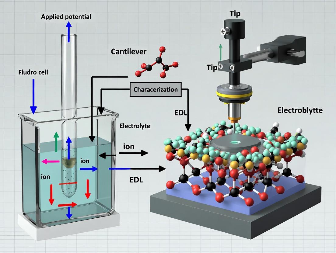
Within the thesis context of 3D Atomic Force Microscopy (3D-AFM) for EDL characterization, understanding the EDL is paramount. 3D-AFM maps force interactions between a nanoscale tip and a sample across three spatial dimensions, directly probing the nanomechanical and electrostatic forces arising from the EDL. This enables the visualization of its structure with sub-nanometer resolution, a capability central to advancing research in material science (e.g., battery interfaces, catalysts) and life sciences (e.g., membrane biophysics, drug delivery systems).

Theoretical Framework: The Structure of the EDL

The classical model (Gouy-Chapman-Stern) divides the EDL into several regions:

• Inner Helmholtz Plane (IHP): The plane through the centers of specifically adsorbed ions (dehydrated, directly bound to the surface).
• Outer Helmholtz Plane (OHP): The plane of closest approach for hydrated counter-ions.
• Diffuse Layer: A region extending from the OHP into the bulk solution where ion concentration decays exponentially, described by the Poisson-Boltzmann equation.

The potential drop across these layers is critical. The zeta potential ((\zeta))—the potential at the shear plane (slightly beyond the OHP)—is a key measurable parameter influencing colloidal behavior and interaction forces.

Quantitative Parameters of the EDL

Table 1: Key EDL Parameters and Their Significance

Parameter	Symbol	Typical Range / Value	Significance
Surface Potential	(\Psi_0)	± 10 - 500 mV	Intrinsic charge of the surface.
Stern Layer Capacitance	(C_{Stern})	10 - 100 µF/cm²	Dielectric properties of the inner, structured layer.
Diffuse Layer Capacitance	(C_{Diff})	Varies with ionic strength	Describes ion distribution in the diffuse layer.
Debye Length	(\kappa^{-1})	~0.3 nm (1M NaCl) to ~100 nm (1e-5M NaCl)	Characteristic thickness of the diffuse layer. Inverse depends on ionic strength ((I)).
Zeta Potential	(\zeta)	± 1 - 100 mV	Practical, measurable potential governing colloidal interactions.

The Debye length ((\kappa^{-1})) is calculated as: [ \kappa^{-1} = \sqrt{\frac{\epsilonr \epsilon0 kB T}{2 NA e^2 I}} ] where (\epsilonr) is relative permittivity, (\epsilon0) vacuum permittivity, (kB) Boltzmann constant, (T) temperature, (NA) Avogadro's number, (e) elementary charge, and (I) ionic strength.

Application Notes: Probing the EDL with 3D-AFM

3D-AFM, specifically 3D force mapping, is a revolutionary technique for EDL characterization. It involves recording force-distance (F-D) curves at every pixel in a 2D scan area, constructing a 3D force volume map ((F(x,y,z))). This map contains the full spatial information of tip-sample interactions, including EDL forces.

Key Applications:

• Mapping Local Surface Potential: By fitting F-D curves with DLVO (Derjaguin-Landau-Verwey-Overbeek) theory or Poisson-Boltzmann models, local variations in surface charge/potential can be quantified.
• Visualizing Ion Distribution: 3D force maps can reveal the spatial organization of ions in the diffuse layer, especially with functionalized tips.
• Biomolecular Interfaces: Studying the role of EDL in protein adsorption, lipid bilayer formation, and ligand-receptor binding in physiologically relevant electrolytes.
• Energy Materials: Characterizing the EDL structure at electrode-electrolyte interfaces in batteries and supercapacitors to inform device design.

Experimental Protocols

Protocol 1: 3D-AFM Force Volume Mapping for EDL Characterization

Objective: To acquire a 3D force map of a charged surface (e.g., mica, functionalized gold) in an electrolyte solution to extract EDL parameters.

Materials: See "The Scientist's Toolkit" below.

Procedure:

• Sample Preparation:
  • Clean substrate (e.g., freshly cleaved mica, plasma-cleaned gold slide) in a laminar flow hood.
  • If functionalization is required (e.g., with self-assembled monolayers, proteins), perform under controlled conditions. Immerse in functionalization solution for specified time, then rinse thoroughly with appropriate solvent and the intended electrolyte.
• AFM Fluid Cell Assembly:
  • Mount the sample onto the AFM metal disk using a small amount of adhesive.
  • Assemble the fluid cell with O-rings, ensuring no leaks. Install the cantilever into the holder.
  • Fill the fluid cell with the desired electrolyte solution (e.g., 1mM to 100mM KCl, PBS), avoiding bubbles.
• System Setup & Thermal Equilibrium:
  • Mount the fluid cell onto the AFM scanner.
  • Allow the system to thermally equilibrate for at least 30 minutes to minimize drift.
  • Engage the tip in contact mode to find the surface, then retract.
• Cantilever Calibration:
  • In fluid, calibrate the cantilever's sensitivity (InvOLS) on a hard, non-deformable area of the sample.
  • Perform thermal tuning to determine the spring constant ((k)) of the cantilever in fluid.
• 3D Force Volume Parameter Setting:
  • Set the scan area (e.g., 500 x 500 nm).
  • Define the pixel resolution (e.g., 64 x 64 pixels).
  • Set the force curve trigger point (e.g., 1-5 nN) to avoid sample damage.
  • Define the Z-scan size (e.g., 50-100 nm) to fully capture the long-range EDL interaction and the repulsive contact region.
  • Set the approach/retract speed (e.g., 100-500 nm/s) to balance data quality and acquisition time.
• Data Acquisition:
  • Initiate the 3D force volume scan. The system will automatically acquire an F-D curve at every pixel.
  • Monitor initial curves for consistency and adjust trigger point or Z-range if necessary.
• Data Processing & Analysis (Post-Experiment):
  • Use specialized software (e.g., Bruker's NanoScope Analysis, Gwyddion, custom Matlab/Python scripts).
  • Baseline Subtraction: Flatten the non-interacting part of all F-D curves.
  • Force Conversion: Convert photodetector voltage to force (nN) using the calibrated sensitivity and spring constant.
  • Tip-Separation Calculation: Correct the Z-piezo displacement for cantilever bending to obtain true tip-sample separation, (D).
  • Model Fitting: Fit the non-contact portion of individual or averaged F-D curves with an EDL model (e.g., constant charge or constant potential model within DLVO framework) to extract local Debye length and surface potential.

Protocol 2: Dynamic Zeta Potential Measurement via AFM (Colloid Probe Method)

Objective: To measure the effective zeta potential of a surface by analyzing the long-range electrostatic interaction with a spherical colloidal probe.

Procedure:

• Colloid Probe Fabrication: Attach a silica or polystyrene microsphere (diameter 2-20 µm) to a tipless AFM cantilever using a micromanipulator and a suitable epoxy resin. Cure fully.
• System Setup: Follow steps 2-4 from Protocol 1, using the colloid probe.
• Force Curve Acquisition: Acquire single or arrays of F-D curves on the sample surface in the electrolyte of interest. Ensure a low approach speed to avoid hydrodynamic effects.
• Data Analysis: Fit the repulsive (or attractive) exponential decay region of the force curve ((F/R) vs. (D), where R is sphere radius) with the equation: (F/R = 2\pi\epsilonr\epsilon0 \kappa \zeta{tip}\zeta{sample} e^{-\kappa D}) (linearized Poisson-Boltzmann approximation for low potential). If the probe's zeta potential ((\zeta{tip})) is known from independent measurement, the sample's zeta potential ((\zeta{sample})) can be calculated directly.

Diagrams

Title: 3D-AFM EDL Characterization Workflow

Title: Electrical Double Layer Structure & Potential Decay

The Scientist's Toolkit

Table 2: Essential Research Reagents and Materials for EDL Studies with 3D-AFM

Item	Function/Description	Example Product/Brand
AFM with Fluid Capability	Instrument capable of force spectroscopy and 3D mapping in liquid.	Bruker Dimension FastScan, Cypher ES, JPK NanoWizard.
Sharp AFM Probes	For high-resolution topography and force mapping. Silicon nitride tips are common for biological work.	Bruker SNL, Olympus RC800PB, NanoWorld Arrow-NCR.
Colloidal Probes	Functionalized microspheres attached to cantilevers for quantitative surface potential measurement.	Novascan colloidal probe kits, custom-fabricated probes.
Ultra-Flat Substrates	Provide atomically smooth reference surfaces for calibration and model studies.	Muscovite Mica (V1 Grade), Highly Oriented Pyrolytic Graphite (HOPG).
Functionalization Chemicals	Modify surface charge/chemistry (e.g., silanes, thiols, polyelectrolytes).	(3-Aminopropyl)triethoxysilane (APTES), 11-Mercaptoundecanoic acid (MUA).
High-Purity Salts	Prepare electrolytes with precise ionic strength and composition.	KCl, NaCl, MgCl₂ (≥99.99% trace metals basis, Sigma-Aldrich).
pH Buffers	Control solution pH, a critical factor for surface charge determination.	Phosphate Buffered Saline (PBS), HEPES, MES buffers.
Deionized/Ultrapure Water	Solvent for all electrolytes; must have high resistivity (>18 MΩ·cm).	Millipore Milli-Q or equivalent system output.
Data Analysis Software	Essential for processing 3D force volume data and fitting interaction models.	Bruker NanoScope Analysis, Igor Pro with custom procedures, Gwyddion, Matlab/Python.

This application note details the evolution from conventional 2D topographic imaging to quantitative 3D force mapping via Atomic Force Microscopy (AFM), specifically framed within a thesis on 3D-AFM for Electrical Double Layer (EDL) characterization. Understanding the 3D structure and properties of the EDL at solid-liquid interfaces is critical for research in biophysics, nanomaterial science, and targeted drug delivery, where interfacial forces govern molecular interactions, adhesion, and stability.

Key Methodological Evolution: From 2D to 3D

2.1 Traditional 2D Topographic AFM

• Mode: Primary contact or tapping mode in air/liquid.
• Output: A height map (x, y, z) representing surface topography.
• Limitation for EDL Studies: Provides only structural information; convolutes true topography with surface forces, and offers no direct quantitative data on the local force fields surrounding a sample.

2.2 3D Force-Volume AFM

• Principle: At each pixel in an (x,y) grid, a full force-distance (F-D) curve is captured by extending and retracting the tip.
• Output: A 3D data cube (x, y, δ), where δ is tip-sample separation, with force as the measured variable.
• Advantage: Decouples topography from force, allowing mapping of interaction forces (e.g., van der Waals, electrostatic, solvation) in all three dimensions.

2.3 Advanced 3D Force Mapping: PinPoint Mode & Fast Spectroscopy

• Evolution: Modern modes separate topographic scanning from force spectroscopy. The tip traces topography via a single feedback channel, then lifts to a defined height at each pixel to perform a rapid F-D curve without lateral shear force.
• Thesis Relevance: This is essential for accurate EDL characterization, as it prevents tip/sample damage and measures pure vertical force fields, enabling the reconstruction of the 3D EDL potential.

Quantitative Comparison of AFM Modes

Mode	Primary Data	Spatial Resolution	Force Sensitivity	Speed (for 128x128 pts)	Key Output for EDL Studies
Contact Mode (2D)	Topography (z)	~1 nm lateral	Low (nN)	1-2 minutes	Surface roughness; indirect inference.
Tapping Mode (2D)	Topography & Phase	~1 nm lateral	Medium (pN-nN)	2-5 minutes	Topography with material contrast.
Force-Volume (3D)	Force vs. Distance Cube	~10-20 nm lateral	High (pN)	10-60 minutes	3D maps of adhesion, stiffness, long-range forces.
PinPoint/Fast 3D (3D)	Separated Topography & F-D Cube	~5-10 nm lateral	Very High (pN)	5-20 minutes	High-resolution, damage-free 3D force maps; direct EDL potential.

Core Protocols for 3D-AFM in EDL Characterization

Protocol 1: 3D Force Mapping in Electrolyte Solutions Objective: To map the 3D electrostatic double layer force around a sample in a controlled ionic environment.

• Sample Preparation: Immobilize the sample (e.g., lipid bilayer, protein, polymer) on a freshly cleaved mica substrate. Load into a liquid cell.
• Probe Selection & Calibration: Use a sharp, conductive AFM tip (e.g., doped diamond, Pt/Ir-coated Si). Calibrate the cantilever's spring constant (k) via thermal tune method. Determine the optical lever sensitivity (InvOLS).
• System Setup: Fill the liquid cell with the desired electrolyte solution (e.g., 1-100 mM KCl, pH-buffered). Allow thermal and mechanical equilibration for 20 minutes.
• Topography Imaging: Acquire a stable, high-resolution topographic image in Peak Force Tapping or AC mode to define the region of interest (ROI).
• 3D Force Map Acquisition:
  • Set the ROI grid size (e.g., 64x64 points).
  • Define the Z-spectroscopy parameters: extend/retract distance (typically 50-100 nm to probe full EDL decay), velocity (100-500 nm/s to minimize viscous drag), and trigger point (or peak force).
  • Engage the PinPoint or Quantitative Imaging (QI) mode. The system will capture a full F-D curve at every pixel, with tip lift between points.
• Data Collection: The system outputs a 3D array of force vs. tip-sample separation data for the entire grid.

Protocol 2: Deconvolution of EDL Force from Total Interaction Objective: To isolate the electrostatic component from the measured total force profile.

• Raw Data Processing: Convert all F-D curves from volts to Newtons using k and InvOLS. Align curves by the point of contact (hard wall repulsion).
• Background Subtraction: In areas far from the sample (e.g., on the substrate), average force curves to define a baseline and subtract it from all curves.
• Force Decomposition: Fit the non-contact region of each processed F-D curve with a composite model: F_total(d) = F_EDL(d) + F_vdW(d) + F_hydration(d)
  • FEDL: Fit using the Poisson-Boltzmann-derived model (e.g., constant charge or constant potential).
  • FvdW: Use a standard Hamaker-form expression (-A*R/(6d^2) for sphere-plane).
  • F_hydration: Use an exponential decay model if present in high-resolution data.
• 3D Parameter Mapping: Extract fitting parameters (e.g., surface potential, charge density, decay length) at each pixel to generate quantitative 3D maps of EDL properties.

The Scientist's Toolkit: Essential Research Reagents & Materials

Item	Function & Relevance to 3D-AFM/EDL
Conductive AFM Probes (e.g., SCM-PIT-V2)	Coated with Pt/Ir for simultaneous electrical and force sensing; crucial for probing electrostatic interactions.
Diamond-Coated Probes (CDT-NCHR)	Extreme wear resistance for prolonged 3D mapping in liquid; consistent tip geometry ensures reliable force data.
Calibration Gratings (TGZ1, PG)	For verifying lateral (XY) and vertical (Z) scanner accuracy, ensuring dimensional fidelity in 3D maps.
Mica Substrates (V1 Grade)	Atomically flat, negatively charged surface for reproducible sample immobilization and EDL measurements.
Standard Buffer Salts (KCl, NaCl)	To prepare electrolytes of precise ionic strength, controlling the Debye length (κ⁻¹) of the EDL.
pH Buffer Solutions (e.g., HEPES, PBS)	To maintain stable and biologically relevant pH, critically affecting surface charge and potential.
Functionalized PEG Linkers	For tethering biomolecules (proteins, DNA) to tips or samples, enabling specific force spectroscopy within 3D maps.

Visualizing the 3D-AFM Workflow & Data Analysis

Title: 3D-AFM Experimental & Analysis Workflow

Title: Force Decomposition for EDL Analysis

Within the broader thesis on 3D atomic force microscopy for Electrical Double Layer (EDL) characterization, this document outlines the core principles, applications, and protocols. 3D-AFM, an advanced scanning probe technique, enables the direct, quantitative mapping of solvated interfaces and nanoscale forces in three dimensions, providing critical insights for surface science, materials research, and drug development.

Core Principles and Quantitative Data

3D-AFM extends traditional AFM by performing a dense 3D raster scan. At each lateral (x, y) point, the tip approaches and retracts from the surface while measuring force, building a 3D force field map. This reveals solvation structures, ion distributions, and biomolecular interactions within the EDL.

Table 1: Key Quantitative Parameters in 3D-AFM for EDL Studies

Parameter	Typical Range/Value	Significance
Z-resolution (vertical)	1 - 10 pm	Resolves atomic corrugation and layered solvation structures.
XY-resolution (lateral)	0.1 - 1 nm	Resolves atomic lattices and molecular-scale features.
Force Sensitivity	1 - 10 pN	Detects weak non-covalent forces (e.g., hydration, van der Waals).
Force Measurement Range	± 1 nN	Covers adhesion, electrostatic, and steric forces.
3D Scan Volume	Up to 10 x 10 x 5 nm³	Captures the extended EDL and molecular adlayers.
Salt Concentration (for EDL)	1 mM - 1 M	Modulates EDL thickness (Debye length: ~0.3 - 10 nm).
Measured Debye Length (1 mM NaCl)	~9.6 nm	Validates theory and probe performance in liquid.

Table 2: Measured Force Magnitudes for Common Interactions

Interaction Type	Typical Force Magnitude	Characteristic Distance Range
Hydration Repulsion	50 - 500 pN	0.3 - 1.5 nm from surface
van der Waals Attraction	100 - 2000 pN	0.5 - 5 nm
Steric/Bumped Repulsion	0.5 - 5 nN	< 1 nm (contact)
Electrostatic (EDL) Force	± 10 - 500 pN	1 - 20 nm (depends on ionic strength)
Specific Adhesion (e.g., ligand-receptor)	50 - 200 pN	Upon retraction (snap-off)

Experimental Protocols

Protocol 1: 3D Force Mapping of the Electrical Double Layer on Mica

Objective: To acquire a 3D force map characterizing the ion distribution and hydration structure over a charged surface in aqueous electrolyte. Materials: See "The Scientist's Toolkit" below. Procedure:

• Substrate Preparation: Cleave a fresh sheet of muscovite mica. Immediately mount it in the liquid cell.
• Liquid Cell Assembly: Fill the cell with the desired electrolyte solution (e.g., 100 mM NaCl). Ensure no air bubbles are trapped.
• Cantilever Selection & Calibration: Use a sharp, conductive probe (e.g., diamond-coated Si). Calibrate the spring constant (k ~ 0.1 - 0.5 N/m) via thermal tune method. Determine the optical lever sensitivity on a hard sapphire surface in liquid.
• System Equilibration: Allow the fluid cell to thermally equilibrate for 30 minutes to minimize drift.
• 2D Approach Curve Grid Definition: Set the lateral scan area (e.g., 5 x 5 nm). Define a pixel array (e.g., 32 x 32 points). Set the Z-scan range to 5-10 nm above the anticipated contact point.
• Data Acquisition Parameters: Set the Z-approach/retract speed to 50-200 nm/s. Sample force at ≥ 512 points per curve. Enable force setpoint feedback to ~100 pN for surface tracking.
• 3D Scan Execution: Initiate the automated 3D scan. The system will acquire a force-distance curve at every (x, y) pixel.
• Data Processing:
  • For each curve, subtract the baseline (non-interacting) force.
  • Align all curves to a common zero-distance using the contact point.
  • Compile processed curves into a 3D array F(x, y, z).
  • Generate 2D slices at constant height or constant force.

Protocol 2: Probing Ligand-Receptor Interactions on a Model Membrane

Objective: To map the binding forces and spatial distribution of a drug candidate (ligand) bound to membrane-embedded receptors. Materials: Supported lipid bilayer (SLB) with incorporated receptors, AFM probe functionalized with specific ligand, relevant buffer. Procedure:

• Probe Functionalization: Incubate a gold-coated tip with a thiolated-PEG linker, followed by the target ligand. Rinse thoroughly.
• Sample Preparation: Form an SLB containing 1-5 mol% of the target receptor protein via vesicle fusion on a silica substrate.
• Buffer Conditions: Use a physiologically relevant buffer (e.g., PBS, pH 7.4).
• 3D Scan Setup: Define a lateral grid over a suspected cell membrane domain (~200 x 200 nm). Set a Z-range of 50 nm.
• Adhesion Mapping: Execute the 3D scan with a moderate approach speed (100 nm/s) and a slow retract speed (50 nm/s) to facilitate binding.
• Analysis: On the retract curves, identify specific adhesion events (characteristic snap-off lengths for PEG linker). Plot the adhesion force magnitude and event probability as 2D maps over the scan area.

Visualizations

Title: 3D-AFM Force Mapping Workflow

Title: 3D-AFM Probes the Electrical Double Layer

The Scientist's Toolkit: Key Research Reagent Solutions

Table 3: Essential Materials for 3D-AFM in EDL/Drug Development Research

Item	Function & Rationale
Ultra-Sharp, Conductive AFM Probes (e.g., diamond-coated Si, Pt/Ir coated)	Essential for high spatial resolution and for applying/measuring electrostatic potentials in electrolyte.
Muscovite Mica Substrates (V1 Grade)	Provides an atomically flat, negatively charged, hydrophilic surface ideal for EDL and biomolecule adsorption studies.
High-Purity Salts (NaCl, KCl, CaCl₂)	To prepare electrolytes of precise ionic strength, modulating EDL thickness and screening.
Functionalization Kits (Thiol-PEG-NHS, silane chemistry)	For covalently attaching specific biomolecules (proteins, ligands, DNA) to AFM tips or substrates.
Supported Lipid Bilayer (SLB) Components (DOPC, cholesterol, functionalized lipids)	To create model cell membranes for probing drug-membrane and receptor-ligand interactions.
Temperature-Controlled Liquid Cell	Maintains physiological or stable experimental conditions, minimizing thermal drift.
Vibration Isolation Platform	Critical for achieving sub-Angstrom vertical resolution by isolating the AFM from building noise.
De-Gassed, Ultrapure Water (≥18.2 MΩ·cm)	Prevents bubble formation under the cantilever and ensures clean electrolyte preparation.

Introduction Within the framework of advancing 3D Atomic Force Microscopy (3D-AFM) for nanoscale interfacial research, the characterization of the Electrical Double Layer (EDL) emerges as a critical parameter. The EDL, the structured region of ions and water molecules at charged surfaces in solution, directly governs molecular interactions in biological systems. Precise mapping of the EDL's 3D potential and ion distribution via 3D-AFM enables predictive insights into three pivotal areas: the kinetics and affinity of drug-target binding, the orientation and density of adsorbed protein coronas on drug delivery vehicles, and the efficiency of nanoparticle cellular uptake. This application note details the quantitative implications and provides protocols for relevant experimental characterization.

Quantitative Data Summary

Table 1: Impact of Surface Potential (ζ-potential) on Biophysical Outcomes

System / Condition	Measured ζ-potential (mV)	Key Outcome	Quantitative Result
Liposome (DPPC:Chol)	-5 ± 2	Protein Adsorption (Fibrinogen)	1200 ± 150 molecules/μm²
Liposome (DPPC:Chol:POPS)	-45 ± 3	Protein Adsorption (Fibrinogen)	280 ± 40 molecules/μm²
Anti-inflammatory Drug (Neutral pH)	+15 ± 5	Binding Constant (Target Enzyme)	Kd = 2.1 ± 0.3 μM
Anti-inflammatory Drug (Acidic pH)	+25 ± 5	Binding Constant (Target Enzyme)	Kd = 0.7 ± 0.1 μM
PEGylated AuNP	-10 ± 3	Cellular Uptake (HeLa cells)	1.2 × 10⁴ particles/cell
Chitosan-coated AuNP	+35 ± 5	Cellular Uptake (HeLa cells)	8.5 × 10⁴ particles/cell

Table 2: 3D-AFM Operational Parameters for EDL Mapping

AFM Mode	Probe Specification	Key Measurement	Buffer Consideration	Resolution (Typical)
3D PeakForce QNM	Silicon nitride, tip radius < 10nm, conductive coating (Pt/Ir)	Local dielectric constant, Debye length	Controlled ionic strength (0.1-100 mM)	Vertical: 0.1 nm, Lateral: 5 nm
Scanning Kelvin Probe Force Microscopy (SKPFM)	Conductive diamond-coated, high resonance frequency	Surface potential (Volta potential)	Requires non-conductive substrate	Potential: 1 mV, Spatial: 20 nm
Frequency-Modulated Electrostatic Force Microscopy (FM-EFM)	Sharp conductive probe (single-electron sensitivity)	Quantitative charge mapping	Ultra-high vacuum or controlled humidity	Charge: <1e, Spatial: 10 nm

Experimental Protocols

Protocol 1: 3D-AFM Mapping of EDL Structure at a Drug-Binding Site Objective: To spatially resolve the ion distribution and potential decay within the EDL over a purified protein target (e.g., kinase enzyme) under varying buffer conditions. Materials: See "The Scientist's Toolkit" below. Procedure:

• Sample Preparation: Immobilize the purified target protein on a freshly cleaved mica substrate using a Ni-NTA functionalization protocol for His-tagged proteins. Rinse gently with appropriate buffer (e.g., 20 mM HEPES, pH 7.4).
• AFM Probe Selection & Calibration: Use a conductive, sharp probe (e.g., PPP-EFM, Nanosensors). Calibrate the spring constant via thermal tune method and sensitivity on a hard sapphire surface.
• 3D Force-Volume Mapping: a. Position the probe above a region of interest on the protein surface. b. Execute a 3D raster scan (e.g., 500 nm x 500 nm x 20 nm grid). At each (x,y) point, perform a force-distance curve with a Z-sweep of 50 nm. c. Operate in PeakForce Tapping mode with a frequency of 0.25-1 kHz to maintain probe integrity.
• Buffer Exchange & Data Acquisition: Flush the fluid cell sequentially with buffers of increasing ionic strength (1 mM, 10 mM, 150 mM KCl in 20 mM HEPES). Acquire a new 3D force map at each condition.
• Data Analysis: Use the Derjaguin-Landau-Verwey-Overbeek (DLVO) theory-based fitting module in the AFM software (e.g., NanoScope Analysis) to extract the local surface potential and Debye length from the force-distance curves at each pixel, constructing 3D EDL potential maps.

Protocol 2: Correlating Nanoparticle EDL Properties with Cellular Uptake Objective: To measure the ζ-potential and EDL-mediated interaction forces of nanoparticles (NPs) and correlate them with quantified cellular internalization. Materials: See "The Scientist's Toolkit" below. Procedure:

• NP Synthesis & Characterization: Synthesize NPs (e.g., AuNPs, polymeric NPs) with controlled surface chemistry. Measure bulk ζ-potential via Dynamic Light Scattering (DLS).
• Single-NP Force Spectroscopy: a. Immobilize NPs on a poly-L-lysine-coated mica substrate. b. Functionalize an AFM cantilever tip with a plasma membrane fragment or a specific cell receptor (using PEG-crosslinker chemistry). c. Approach the functionalized tip to individual immobilized NPs in relevant cell culture medium. Record force-distance curves at multiple approach/retract cycles. d. Analyze the adhesion force, jump-in distance (related to EDL range), and work of adhesion from retraction curves.
• Cellular Uptake Quantification: a. Incubate fluorescently labeled NPs with cells (e.g., HeLa, HEK293) in a 12-well plate for 4 hours at 37°C. b. Wash cells extensively with glycine buffer (pH 2.5) to remove membrane-bound NPs. c. Lyse cells and measure fluorescence intensity with a plate reader. Use a standard curve to calculate the number of NPs internalized per cell.
• Data Correlation: Plot NP uptake (particles/cell) against both bulk ζ-potential and the average adhesion force measured via AFM to establish structure-activity relationships.

Visualizations

Title: 3D-AFM EDL Workflow to Biophysical Implications

Title: How EDL Compression Enhances Drug Binding

The Scientist's Toolkit

Table 3: Essential Research Reagents & Materials for EDL Characterization

Item	Function in EDL Research
Conductive AFM Probes (Pt/Ir or Diamond Coated)	Enables simultaneous topographical imaging and electrostatic potential measurement (SKPFM, EFM).
Functionalization Kits (e.g., Ni-NTA, PEG Crosslinkers)	For immobilizing proteins or biomolecules on AFM tips and substrates with controlled orientation.
Ionic Strength Buffer Kits (KCl/HEPES)	To systematically vary Debye length (λ_D = 0.304/√I nm) and probe EDL compression effects.
Standard Reference Samples (e.g., HOPG, Sapphire)	For AFM probe calibration and verification of electrostatic force measurements.
ζ-potential Reference Materials (e.g., Latex Beads)	To validate and calibrate bulk ζ-potential measurements from DLS instruments.
Fluorescent Nanoparticle Tracking Analysis (NTA) Kit	To correlate NP size, concentration, and ζ-potential with cellular uptake data.
Microfluidic AFM Liquid Cells (Temperature Controlled)	Allows stable, prolonged 3D-AFM imaging and force mapping under buffer exchange.
DLVO Theory Analysis Software Module	Essential for fitting force-distance curves to extract surface charge and Hamaker constants.

Key Components of a Modern 3D-AFM Setup for Bio-Interface Studies

Within the broader thesis on 3D atomic force microscopy for Electric Double Layer (EDL) characterization at biological interfaces, this document details the essential components and protocols for a modern 3D-AFM setup. The ability to probe bio-interfaces—such as protein-membrane, cell-substrate, or drug-receptor interactions—in three dimensions with nanoscale resolution is critical for advancing fundamental biophysics and drug development.

Key Components of a Modern 3D-AFM Setup

A state-of-the-art 3D-AFM system for bio-interface studies integrates advanced hardware, environmental control, and specialized software to enable precise, non-destructive 3D nanoscale imaging and force spectroscopy in liquid.

Table 1: Core Hardware Components of a 3D-AFM Setup

Component	Specification/Model Example	Function in Bio-Interface Studies
AFM Head & Scanner	High-resolution piezo scanner (e.g., XYZ closed-loop); range: ≥100µm XY, 15µm Z.	Provides precise 3D positioning of tip relative to sample. Closed-loop control ensures accuracy for volume reconstruction.
Cantilever & Probe	Ultrashort, stiff cantilevers (e.g., BL-AC40TS, k≈0.1 N/m, f₀≈30 kHz in liquid); functionalized tips.	Minimizes hydrodynamic drag for 3D mapping. Functionalization (e.g., with PEG linkers) enables specific molecular recognition.
Liquid Cell	Sealed fluid cell with temperature control (±0.1°C) and perfusion inlets/outlets.	Maintains physiological conditions, allows buffer exchange, and controls ionic strength for EDL studies.
Vibration & Acoustic Isolation	Active anti-vibration table with acoustic enclosure.	Isolates system from ambient noise critical for high-resolution imaging in soft biological modes.
Environmental Chamber	Humidity (>80%) and CO₂ (5%) control.	Essential for long-term live-cell imaging studies.
Detection System	Highly sensitive photodetector (quadrant photodiode) with low-noise laser.	Measures cantilever deflection (<10 pN force sensitivity) for topography and force detection.
Control Electronics & Software	High-speed digital controller; 3D-AFM specific software (e.g., cAFM, 3D Force Map modules).	Executes 3D scanning protocols, data acquisition, and real-time analysis.

Table 2: Key Software & Analytical Modules

Module/Technique	Key Parameter	Application in Bio-Interface/EDL Research
3D Force Volume Mapping	Pixel array: 128x128; Z-points: 64-128; acquisition rate: 1-5 Hz/pixel.	Acquires full force-distance curves at each pixel, building a 3D data cube of tip-sample interaction forces.
PeakForce Tapping 3D Mode	Oscillation frequency: 0.5-2 kHz; peak force setpoint: 50-200 pN.	Enables high-resolution, gentle imaging of soft samples (proteins, membranes) with simultaneous nanomechanical mapping.
Digital Pulsed Force Mode (DPFM)	Pulse frequency: 0.5-5 kHz.	Provides high-speed viscoelastic mapping, ideal for heterogeneous biological surfaces.
3D Data Reconstruction Software	Deconvolution algorithms (e.g., inverse point spread function).	Reconstructs true 3D distribution of mechanical/chemical properties from the force volume data cube.
EDL & DLVO Fitting Libraries	Poisson-Boltzmann solvers; Hamaker constant databases.	Quantifies electrostatic and van der Waals forces from force spectroscopy data to characterize the EDL.

Experimental Protocols for Bio-Interface Characterization

Protocol 3.1: 3D EDL Mapping on a Supported Lipid Bilayer (SLB)

Objective: To map the 3D structure of the Electric Double Layer above a model membrane under varying ionic strength conditions.

Materials:

• SLB Sample: DOPC or DOPC/DOPS bilayers formed via vesicle fusion on mica.
• Buffers: 10 mM, 50 mM, and 150 mM KCl in 10 mM HEPES (pH 7.4).
• AFM Probe: Sharp, non-functionalized silicon nitride tip (e.g., SNL-10).

Procedure:

• System Setup: Mount the liquid cell, inject 10 mM KCl buffer, and allow thermal equilibration (≥30 min).
• Probe Engagement: Engage the cantilever in liquid at a low setpoint (0.5 nN) using standard contact mode.
• 3D Force Volume Acquisition:
  • Set a scan area (e.g., 1 x 1 µm²) with 64x64 pixels.
  • Define a Z-sweep distance of 50 nm (extending well beyond the EDL decay length).
  • Set Z-sweep frequency to 2 Hz.
  • Initiate the 3D scan. The system automatically acquires a force-distance curve at every pixel.
• Buffer Exchange: Perfuse the cell gently with 50 mM, then 150 mM KCl buffers, repeating step 3 for each condition.
• Data Analysis:
  • Use software to convert deflection vs. Z-piezo data to force vs. true tip-sample separation for all curves.
  • At each pixel, fit the non-contact portion of the force curve (typically exponential decay) to a Poisson-Boltzmann model to extract local surface potential (ψ) and Debye length (κ⁻¹).
  • Reconstruct 2D maps of ψ and κ⁻¹ for each buffer condition.

Protocol 3.2: Molecular Recognition Imaging (TREC) in 3D

Objective: To locate and visualize the 3D distribution of specific receptors (e.g., EGFR) on a live cell surface.

Materials:

• Sample: Live epithelial cells (A431 line) cultured on a glass-bottom Petri dish.
• Functionalized Probe: Cantilever tipped with an anti-EGFR antibody via a flexible PEG crosslinker.
• Imaging Buffer: Phenol-red free cell culture medium at 37°C.

Procedure:

• Sample Mounting: Place the petri dish in the AFM stage heater, maintaining 37°C and 5% CO₂.
• Probe Alignment: Align the laser on the functionalized cantilever in air, then mount in the fluid cell.
• Engagement and Imaging:
  • Inject medium, engage on a cell-free area using PeakForce Tapping mode (Peak Force ≈150 pN, frequency 1 kHz).
  • Navigate to a cell of interest.
  • Initiate a 3D PeakForce QNM scan: The system records topography, adhesion force, deformation, and dissipation maps simultaneously.
  • The adhesion map highlights specific antibody-receptor binding events as distinct, high-adhesion pixels.
• Control Blocking Experiment: Add a high concentration of free anti-EGFR antibody to the medium to competitively block receptors. Repeat scan. The specific adhesion signal should vanish.
• 3D Reconstruction: Combine sequential adhesion maps from Z-stacks (achieved by varying the setpoint) to generate a 3D volume rendering of receptor distribution on the cell surface.

The Scientist's Toolkit: Research Reagent Solutions

Table 3: Essential Materials for 3D-AFM Bio-Interface Studies

Item	Function & Rationale
Mica Disks (V1 Grade)	An atomically flat, negatively charged substrate for adsorbing biomolecules (proteins, DNA) or forming supported lipid bilayers.
PEG Crosslinkers (e.g., NHS-PEG-NHS)	A flexible, inert spacer for tip functionalization. It separates the biomolecular ligand from the tip surface, allowing proper orientation and reducing nonspecific binding.
Lipids for SLBs (e.g., DOPC, DOPS, Cholesterol)	Building blocks for creating stable, fluid model membranes to study membrane-protein interactions and electrostatic properties.
BSA (Bovine Serum Albumin)	Used as a blocking agent to passivate AFM tips and fluid cell components, minimizing nonspecific adsorption.
Buffers with Controlled Ionic Strength (e.g., HEPES-KCl)	Allow systematic variation of Debye length to probe EDL forces and mimic physiological conditions.
Calibration Gratings (e.g., TGZ1, TGXY01)	Standard samples with known pitch and height for verifying scanner accuracy in X, Y, and Z dimensions.
Cantilever Calibration Kit	Contains reference cantilevers of known spring constant for accurate calibration of the experimental cantilever's sensitivity and spring constant via thermal tune method.

Visualization of Workflows and Relationships

Title: 3D-AFM Bio-Interface Experiment Workflow

Title: Component Interaction for Bio-Insights

Protocols in Practice: A Step-by-Step Guide to 3D-AFM for Bio-EDL Mapping

Within the broader thesis on 3D Atomic Force Microscopy (3D-AFM) for Electrical Double Layer (EDL) characterization, sample preparation is the critical determinant of experimental success. Accurate 3D-AFM mapping of local electrostatic potentials, hydration structures, and mechanical properties at the solid-liquid interface requires atomically flat, chemically defined biomimetic surfaces and viable, adherent live cells. This document outlines standardized protocols to achieve such pristine samples, ensuring reproducible and high-fidelity data for biophysical and pharmacological research.

Biomimetic Surface Preparation for EDL Characterization

Biomimetic surfaces, such as supported lipid bilayers (SLBs) and self-assembled monolayers (SAMs), provide a simplified, controlled model of cellular membranes.

Protocol: Fabrication of Mica-Supported Lipid Bilayers (SLBs)

• Objective: Create a fluid, defect-free planar SLB on atomically flat mica for 3D-AFM studies of EDL properties over varying lipid headgroups.
• Materials: High-grade muscovite mica, vesicles of desired lipid composition (e.g., DOPC, DOPG, DOPS), buffer (e.g., 150 mM NaCl, 10 mM HEPES, 2 mM CaCl2, pH 7.4), temperature-controlled bath sonicator, and extrusion setup.
• Procedure:
  • Mica Substrate: Cleave mica with fresh, adhesive tape to obtain an atomically flat surface. Immediately mount in the AFM fluid cell.
  • Small Unilamellar Vesicle (SUV) Preparation:
    • Dissolve lipids in chloroform, dry under nitrogen, and desiccate under vacuum for >1 hour.
    • Hydrate the lipid film in appropriate buffer to a final concentration of 0.5 mg/mL.
    • Vortex vigorously, then sonicate in a bath sonicator above the lipid phase transition temperature until the solution clarifies (~30-60 min). Optionally, extrude through a 50 nm polycarbonate membrane 21 times.
  • Bilayer Formation: Inject the SUV suspension into the AFM fluid cell atop the mica. Incubate for 10-15 minutes at a temperature above the lipid phase transition.
  • Rinsing: Gently rinse with 20 mL of measurement buffer to remove excess vesicles and calcium, leaving a fused SLB.
  • Validation: Perform AFM contact mode imaging in fluid to confirm bilayer coverage and fluidity via nanoscale defect imaging.

Key Research Reagent Solutions for Biomimetic Surfaces

Reagent/Material	Function in 3D-AFM/EDL Context
Muscovite Mica (V-1 Grade)	Provides an atomically flat, negatively charged substrate for SLB formation or molecular adsorption. Essential for baseline EDL measurements.
1,2-dioleoyl-sn-glycero-3-phosphocholine (DOPC)	Neutral, zwitterionic lipid forming fluid bilayers. Serves as the baseline model membrane.
1,2-dioleoyl-sn-glycero-3-phospho-L-serine (DOPS)	Lipid with negatively charged headgroup. Used to introduce surface charge for modulating EDL properties.
11-Mercapto-1-undecanol (MUO) SAM on Gold	Creates a hydrophilic, hydroxyl-terminated surface for studying EDL and hydration forces.
16-Mercaptohexadecanoic acid (MHDA) SAM on Gold	Creates a negatively charged, carboxylate-terminated surface for cation-specific EDL studies.

Quantitative Parameters for SLB Quality Control

Table 1: Target Metrics for High-Quality Supported Lipid Bilayers.

Parameter	Target Value	Measurement Technique
Bilayer Thickness	4.5 - 5.5 nm	AFM line profile across a fabricated defect.
Root-Mean-Square (RMS) Roughness	< 0.3 nm (over 1 µm²)	AFM topographic imaging in fluid.
Lateral Diffusion Coefficient (Dₗ)	1 - 5 µm²/s (for fluid phases)	Fluorescence Recovery After Photobleaching (FRAP).
Defect Density	< 0.1% of total area	Statistical analysis of AFM images.

Live Cell Preparation for 3D-AFM

The goal is to maintain cells in a fully viable, morphologically intact, and adherent state during AFM scanning in physiological buffers.

Protocol: Adherent Mammalian Cell Preparation for Long-Duration 3D-AFM

• Objective: Culture and prepare adherent cells (e.g., HEK293, MDCK) for 3D-AFM experiments measuring dynamic EDL and topographical changes.
• Materials: Sterile glass-bottom dishes (pre-coated with Poly-L-Lysine or Collagen), complete cell culture medium, HEPES-buffered imaging medium (e.g., Leibovitz's L-15), pre-warmed PBS, and a temperature-controlled stage.
• Procedure:
  • Substrate Preparation: Coat glass-bottom dishes with appropriate adhesion factor (e.g., 0.1 mg/mL Poly-L-Lysine for 20 min). Rinse thoroughly with sterile water and air dry.
  • Cell Seeding: Seed cells at a low density (~30-40% confluence) 24-48 hours prior to experiment to ensure isolated, well-spread cells.
  • Pre-Experiment (Biosafety Cabinet): On the day of imaging, gently rinse cells once with pre-warmed, serum-free imaging medium (L-15).
  • Medium Exchange: Replace culture medium with 2 mL of pre-equilibrated L-15 imaging medium (no phenol red, with 10% FBS if needed for viability).
  • Mounting: Secure the dish on the AFM stage pre-warmed to 37°C. Allow 15-20 minutes for thermal equilibration and cell settling.
  • Tip Sterilization: Immerse the AFM probe in 70% ethanol for 15 minutes, then rinse thoroughly in sterile PBS and imaging medium before mounting.

The Scientist's Toolkit: Essential Materials for Live-Cell AFM

Reagent/Material	Function in 3D-AFM/EDL Context
Leibovitz's L-15 Medium	CO₂-independent imaging buffer maintains pH without a controlled atmosphere, crucial for open-fluid cell AFM.
Poly-L-Lysine Solution	Promotes strong cell adhesion to glass/mica, preventing detachment during scanning.
Collagen I, Rat Tail	Provides a physiological adhesion substrate for epithelial and endothelial cells.
Biolever Mini or Quantitative Imaging (QI) Probes	Soft cantilevers (k ~0.1 N/m) with sharp tips for low-force, high-resolution live-cell imaging.
Cell Viability Stain (e.g., Calcein-AM)	Fluorescent stain used post-scanning to confirm plasma membrane integrity and viability.

Critical Parameters for Live-Cell Viability

Table 2: Monitoring Parameters for Live-Cell 3D-AFM Experiments.

Parameter	Optimal Condition / Target	Assessment Method
Confluence at Seeding	30-40%	Microscopy inspection pre-mounting.
Medium Osmolarity	290 - 310 mOsm/kg	Osmometer measurement.
Scanning Force	< 100 pN (for soft cells)	Set via AFM force setpoint, monitor cell indentation.
Post-Experiment Viability	> 95%	Calcein-AM / Ethidium Homodimer-1 assay.
Morphological Stability	Consistent height/span over 1 hour	Time-lapse AFM or optical imaging.

Visualization of Workflows

Title: Biomimetic Surface Preparation and QC Workflow

Title: Live Cell Preparation for 3D-AFM Workflow

Selecting and Functionalizing AFM Probes for Optimal EDL Sensitivity

Within the broader thesis on 3D atomic force microscopy (3D-AFM) for electrical double layer (EDL) characterization, the selection and functionalization of the atomic force microscope probe is the single most critical experimental parameter determining sensitivity, resolution, and quantitative accuracy. The EDL, comprising the Stern and diffuse layers of counter-ions at any solid-liquid interface, governs phenomena central to biophysics and drug development, including protein adsorption, membrane potential, and targeted drug delivery. This protocol details the steps for choosing and chemically modifying AFM probes to maximize their sensitivity to localized electrostatic potentials, forces, and ion densities within the EDL in aqueous environments.

Key Considerations for Probe Selection

The probe must balance mechanical, electrical, and geometrical properties. The following table summarizes the critical parameters for optimal EDL sensitivity.

Table 1: Quantitative Comparison of AFM Probe Types for EDL Studies

Probe Type / Coating	Typical Spring Constant (k)	Typical Resonant Frequency (f₀) in Fluid	Typical Radius of Curvature (R)	Conductive Layer (Thickness)	Key Advantage for EDL	Primary Limitation
Si (uncoated)	0.1 - 0.4 N/m	10 - 30 kHz	5 - 10 nm	N/A	High topographical resolution, low cost	Insulating, non-functionalizable Si-OH surface
Si₃N₄ (uncoated)	0.06 - 0.6 N/m	6 - 40 kHz	20 - 60 nm	N/A	Low k for force spectroscopy, biocompatible	Highly insulating, large R, variable surface charge
Pt/Ir coated Si	0.5 - 4 N/m	20 - 75 kHz	20 - 30 nm	10 - 30 nm Pt/Ir	Good conductivity for EFM/KPFM in fluid	Coating increases R, can delaminate, high k
Doped Diamond	1 - 5 N/m	50 - 150 kHz	< 20 nm	Bulk conductive	Extreme durability, stable electrochemistry	Very high k, expensive, limited functionalization
Carbon Nanotube (CNT) tip	0.1 - 1 N/m*	Highly variable	2 - 10 nm (tube end)	Inherently conductive	Atomic-scale R, high aspect ratio, functionalizable	Fragile, challenging attachment, complex dynamics
qPlus Sensor (for 3D-AFM)	1,800 - 10,000 N/m	20 - 50 kHz (tuning fork)	< 10 nm (attached wire)	Pt/Ir wire	Enables true atomic resolution, 3D force mapping	Extremely high k, specialized hardware required

*Effective k depends on CNT length and attachment.

Selection Protocol:

• Define Measurement Mode: For 3D-AFM/Force Volume Mapping, use soft Si or Si₃N₃ probes (k ≈ 0.1-0.2 N/m) to minimize sample deformation during grid-based force-distance acquisition. For Electrostatic Force Microscopy (EFM) in liquid, a conductive Pt/Ir-coated probe is mandatory.
• Minimize Radius of Curvature (R): Select the sharpest available probe (R < 10 nm ideal) to achieve high spatial resolution of localized EDL potentials. CNT or high-quality doped diamond tips are optimal.
• Optimize Spring Constant: Choose the softest possible cantilever (lowest k) compatible with your sample's stiffness to maximize force sensitivity to the weak, exponentially decaying EDL forces (typically 10-100 pN).
• Verify Coating Stability: If using a coated conductive probe, consult manufacturer data or literature to confirm the coating's electrochemical stability in your intended buffer solution (e.g., pH, ionic strength) to avoid drift and artifacts.

Probe Functionalization Protocols

Functionalization tailors the probe's chemical terminus, enabling specific electrostatic or molecular recognition interactions with the EDL.

Protocol 3.1: Silanization for Terminal Amine (-NH₂) or Carboxyl (-COOH) Groups

Purpose: Creates a chemically stable, covalently bonded monolayer on SiO₂ or Si₃N₄ tips for subsequent biomolecule attachment or charge modification. Materials: APTES ((3-Aminopropyl)triethoxysilane), MPTMS (3-Mercaptopropyltrimethoxysilane), absolute ethanol, anhydrous toluene, acetic acid. Procedure:

• Cleaning: Plasma clean probe for 2-3 minutes to create a hydrophilic, OH-rich surface.
• Solution Preparation: For -NH₂ groups, prepare 2% (v/v) APTES in anhydrous toluene. For -SH groups (later oxidized to -COOH), prepare 2% MPTMS in anhydrous toluene. Add a few drops of acetic acid (APTES) or triethylamine (MPTMS) as a catalyst.
• Reaction: Immerse the probe in the silane solution under nitrogen atmosphere for 2 hours at room temperature.
• Rinsing: Rinse sequentially with fresh toluene, ethanol, and Milli-Q water to remove physisorbed silane.
• Curing: Bake at 110°C for 30 minutes to complete the condensation reaction.
• Oxidation (for -COOH from -SH): Immerse MPTMS-functionalized probe in a 30% H₂O₂ solution for 1 hour to oxidize terminal thiols to sulfonic/carboxylic acids. Rinse thoroughly with water.

Protocol 3.2: Thiol-Gold Bonding for Specific Molecule Attachment

Purpose: To attach a specific charged molecule (e.g., a peptide, functional group) or biomarker (e.g., an antibody fragment) to a gold-coated probe with precise orientation. Materials: Gold-coated AFM probe, 1-Octadecanethiol (ODT) or specific thiolated molecule (e.g., HS-(CH₂)₆-COOH, HS-(CH₂)₁₁-NH₂), absolute ethanol. Procedure:

• Cleaning: Clean gold-coated probe by UV-ozone treatment for 15 minutes.
• Functionalization: Immerse the probe in a 1 mM solution of the desired thiolated molecule in ethanol for 12-18 hours at 4°C.
• Rinsing and Drying: Rinse copiously with ethanol and dry under a gentle stream of nitrogen or argon.
• Backfilling (Optional but Recommended): To minimize nonspecific adhesion, immerse the tip in a 1 mM solution of a shorter, inert thiol (e.g., 6-mercapto-1-hexanol) for 30 minutes to backfill any pinholes in the self-assembled monolayer.

Protocol 3.3: PEG Spacer Attachment for Biomolecular Recognition

Purpose: To attach a specific ligand (e.g., a drug molecule, peptide) via a flexible poly(ethylene glycol) (PEG) crosslinker, separating it from the tip surface to allow for natural orientation and reduce steric hindrance during EDL measurements near a functional membrane. Materials: Amine-functionalized probe (from Protocol 3.1), heterobifunctional PEG crosslinker (e.g., NHS-PEG-Maleimide), ligand with appropriate reactive group (thiol for maleimide). Procedure:

• Activation: Dissolve NHS-PEG-Maleimide (MW 3400) in dry DMSO or buffer (pH 7.4) to 5-10 mg/mL. Incubate the amine-functionalized probe in this solution for 1 hour at room temperature. The NHS ester reacts with the terminal amine on the tip.
• Rinsing: Rinse with coupling buffer (e.g., PBS, pH 7.4) to stop the reaction and remove unreacted crosslinker.
• Ligand Coupling: Immediately incubate the activated probe with the thiol-containing ligand solution (50-100 µM in coupling buffer, optionally with a reducing agent like TCEP) for 1-2 hours. The maleimide group reacts specifically with the thiol.
• Quenching: To passivate unreacted maleimide groups, incubate the tip in a 10 mM cysteine solution for 10 minutes.
• Final Rinse: Rinse thoroughly with measurement buffer.

Validation and Calibration Protocols

Protocol 4.1: Quantitative Electrostatic Sensitivity Calibration Purpose: To determine the probe's sensitivity to surface potential (∂F/∂V) before EDL experiments. Procedure:

• Use a sample with a known, stable potential (e.g., highly ordered pyrolytic graphite (HOPG) or a patterned metal electrode) in a controlled humidity environment or fluid cell.
• Perform force-distance spectroscopy or EFM frequency shift measurements while applying a known DC bias (V_dc) between the probe and substrate.
• Fit the resulting force vs. Vdc data at a fixed distance to a parabolic curve: F ∝ (Vdc - Vcpd)², where Vcpd is the contact potential difference. The curvature of the parabola gives ∂²F/∂V², a measure of electrostatic sensitivity.

Protocol 4.2: Functional Group Charge Validation via Force Spectroscopy Purpose: To confirm the successful attachment and charge state of a functional group (e.g., -COOH, -NH₃⁺) by measuring the pH-dependent adhesion with a charged surface. Procedure:

• Use a standardized sample such as a clean silica surface (negatively charged at pH > 2) or an amine-coated surface.
• Perform force-distance curve measurements in buffers of varying pH (e.g., 4, 7, 10) but constant ionic strength (e.g., 10 mM KCl).
• Measure the adhesion force (pull-off force) in each condition. A -COOH functionalized tip will show strong adhesion to an amine surface at low pH (COOH neutral) and weak adhesion at high pH (COO⁻ charged, repulsion from negative silica). The reversal point indicates the pKa of the surface group.

The Scientist's Toolkit: Research Reagent Solutions

Table 2: Essential Materials for AFM Probe Functionalization in EDL Research

Item	Function & Rationale
APTES ((3-Aminopropyl)triethoxysilane)	Creates a stable amine-terminated monolayer on oxide surfaces for subsequent covalent biomolecule attachment or direct use as a positively charged tip at neutral pH.
MPTMS & H₂O₂	MPTMS forms a thiol-terminated monolayer; subsequent oxidation with H₂O₂ creates a stable, negatively charged sulfonic/carboxylic acid surface for anion sensitivity studies.
Heterobifunctional PEG Crosslinkers (e.g., NHS-PEG-Maleimide)	Provides a flexible, inert spacer to attach specific biomolecules (drugs, peptides) to the tip, minimizing nonspecific steric and adhesion forces during EDL probing.
Thiolated Charged Molecules (e.g., HS-C11-COOH, HS-C11-NH₂)	Forms ordered, dense charged monolayers on gold-coated probes via Au-S bonds, enabling well-defined, reproducible surface charge for quantitative EDL modeling.
1-Octadecanethiol (ODT)	Forms a dense, hydrophobic, and electrically insulating monolayer on gold. Used to create chemically inert reference probes or to passivate the sides of conductive tips.
TCEP (Tris(2-carboxyethyl)phosphine)	A reducing agent used to cleave disulfide bonds and maintain thiolated ligands in their reactive (-SH) state during coupling to maleimide-activated tips.
Plasma Cleaner	Critical for generating a clean, hydrophilic, and hydroxylated tip surface prior to silanization, ensuring uniform, covalent monolayer formation.
pH & Ionic Strength Buffers (e.g., PBS, HEPES, citrate)	Essential for controlling the Debye length (κ⁻¹) and the ionization state of tip and sample functional groups during EDL force measurements.

AFM Probe Selection and Functionalization Workflow

Interaction Between Functionalized Tip and Sample EDL

Within the broader thesis on 3D Atomic Force Microscopy (3D-AFM) for Electrical Double Layer (EDL) characterization, this protocol details the design of a 3D Force Volume (FV) experiment. This technique is critical for mapping the 3D force field above a sample surface in liquid, enabling the quantification of local electrostatic, hydration, and steric interactions that define the EDL. Accurate characterization is paramount for research in biophysics, materials science, and drug development, where surface potential and nanoscale interactions dictate function.

The design hinges on optimizing interdependent parameters to balance spatial resolution, force sensitivity, and acquisition time.

Table 1: Primary 3D Force Volume Experiment Parameters

Parameter	Typical Range / Value	Impact on Experiment	Optimization Consideration
Pixel Resolution (XY)	64x64 to 256x256	Defines in-plane spatial resolution. Higher values increase detail but prolong acquisition.	Match to feature size; 128x128 often provides a good compromise.
Z-Scan Range	10 - 100 nm	Depth of force field mapping. Must encompass full EDL decay.	Set based on Debye length (for ionic strength) and expected interaction range.
Z-Points per Curve	64 - 256	Vertical resolution of the force curve. Higher values reveal finer features in the EDL.	128-192 points are typical for resolving hydration layering.
Trigger Point	Set in Attractive regime (e.g., -50 to -100 pN) or Relative trigger (e.g., 5-10 nm above contact)	Determines the closest approach point for each curve. Critical for preserving tip/sample integrity and consistent data.	Use a relative trigger (nm) for soft samples; force trigger for rigid surfaces.
Scan Rate (Approach/Retract Speed)	0.5 - 2 Hz (per curve)	Affects data quality and hydrodynamic forces. Faster speeds reduce acquisition time but can distort force profiles.	Slower speeds (0.5-1 Hz) are essential for accurate EDL measurement near surfaces.
Applied Force Setpoint	50 - 500 pN	Maximum compressive load applied at each pixel.	Use the minimum force necessary to detect repulsion to avoid sample deformation.
Cantilever Spring Constant (k)	0.01 - 0.6 N/m	Determines force sensitivity. Softer levers offer better sensitivity for weak forces.	Calibrate accurately (thermal tune). Use k ~0.1 N/m for biological samples in liquid.
Tip Geometry & Coating	Sharpened Si3N4, SiO2, or Diamond-like Carbon (DLC) coated; Tip radius < 10 nm preferred.	Defines lateral resolution and chemical specificity of interaction.	Use DLC or inert coatings (SiO2) for consistent electrostatic measurements; functionalize for specific interactions.

Table 2: Buffer Composition Impact on EDL & Experimental Settings

Buffer Parameter	Effect on EDL (Debye Length, κ⁻¹)	Recommended 3D-FV Adjustment
Ionic Strength (I)	κ⁻¹ ≈ 0.304/√I nm (for 1:1 electrolyte at 25°C). High I screens potentials, shortens EDL range.	Lower I (1-10 mM) expands EDL, making it easier to map. Use to accentuate electrostatic forces.
pH	Affects surface charge density of sample and tip via protonation/deprotonation.	Buffer away from sample's/isoelectric point (pI) to ensure stable surface charge. Use 10 mM HEPES or PBS.
Divalent Ions (e.g., Mg²⁺, Ca²⁺)	Strong screening and potential specific adsorption, leading to EDL collapse or charge reversal.	Use with caution. Start with monovalent salts (KCl, NaCl) for fundamental EDL characterization.
Additives (e.g., surfactants, polymers)	Can adsorb to tip/sample, altering interfacial properties and masking EDL forces.	Purify buffers; run control experiments in simple electrolyte first.

Detailed Experimental Protocol: 3D Force Volume for EDL Mapping

Objective: To acquire a 3D matrix of force-distance (F-d) curves over a defined XY area and Z-range above a sample surface in a controlled buffer, enabling reconstruction of the 3D force field related to EDL properties.

Materials & Reagent Toolkit:

Table 3: Research Reagent Solutions & Essential Materials

Item	Function in Experiment
AFM with Liquid Cell	Enables imaging and force spectroscopy in a controlled fluid environment. Must have low thermal drift and acoustic noise.
Cantilever & Probe	Force sensor. Choice of spring constant, tip radius, and coating dictates sensitivity and interaction type (see Table 1).
Sample Substrate	Ultra-flat surface (e.g., freshly cleaved mica, gold-coated silicon) with immobilized sample (e.g., lipid bilayer, protein).
Buffer Solutions	Define the electrolyte environment. Includes salt (KCl), pH buffer (HEPES, Tris), and potential chelators (EDTA). Prepare with ultrapure water (18.2 MΩ·cm).
Calibration Gratings	Used for tip characterization (scanning electron microscopy post-experiment recommended) and scanner calibration in Z.
Vibration Isolation Table	Critical for stable, low-noise force measurements at the pN scale.
Fluidic Syringe System	For buffer exchange in the liquid cell without disturbing the tip-sample engagement.

Procedure:

Part A: Preparation (Day 1)

• Sample Preparation: Immobilize your target molecule (e.g., a supported lipid bilayer, self-assembled monolayer, or protein) on an atomically flat substrate (e.g., mica). Verify homogeneity via standard 2D-AFM imaging in fluid if possible.
• Cantilever Preparation:
  • Select a cantilever with an appropriate spring constant (k ≈ 0.1 N/m).
  • Clean the cantilever in an UV-ozone cleaner for 15-20 minutes to remove organic contaminants.
  • (Optional) Functionalize the tip with a specific coating (e.g., SiO2 for silanol groups, DLC for inertness) or molecule following established protocols.
• Buffer Preparation: Prepare the desired electrolyte solution (e.g., 10 mM KCl, 10 mM HEPES, pH 7.4). Filter through a 0.02 µm syringe filter and degas for 30 minutes to prevent bubble formation in the fluid cell.

Part B: System Setup & Calibration (Day 2)

• Mounting: Mount the sample in the liquid cell. Install the prepared cantilever into the holder.
• Wetting: Carefully introduce 50-100 µL of the prepared buffer into the liquid cell to wet the cantilever and sample without engaging.
• Laser Alignment: Align the laser on the back of the cantilever and maximize the sum signal. Adjust the photodiode to center the deflection signal.
• Thermal Tuning: Perform a thermal noise spectrum analysis in fluid to determine the precise spring constant (k) and the optical lever sensitivity (InvOLS, in nm/V) of the cantilever in situ. This is critical for accurate force measurement.
• Approach & Engage: Slowly approach the tip to the sample surface. Engage using a very low setpoint (e.g., -50 pN) to achieve gentle contact.

Part C: 2D Scan and Region Selection

• Perform a standard contact-mode or amplitude-modulation AFM scan in fluid (e.g., 5 µm x 5 µm, 256x256 pixels) to identify a representative, flat region of interest (ROI).
• Zoom into a smaller, featureless area (e.g., 500 nm x 500 nm) for the 3D FV experiment to minimize topographical crosstalk in the force data.

Part D: 3D Force Volume Acquisition

• Parameter Configuration in AFM Software:
  • Set the XY pixel grid (e.g., 64x64 over the 500 nm x 500 nm ROI).
  • Define the Z-scan range (e.g., 50 nm). This range should start from a point where no interaction is felt (tip far from surface) and extend to a point beyond the trigger point.
  • Set the number of Z-points per curve (e.g., 128).
  • Set the trigger point. For EDL mapping on a rigid surface, a force trigger of -100 pN (slight attractive setpoint) is recommended to consistently define the point of closest approach.
  • Set the approach/retract speed (e.g., 0.8 Hz, corresponding to ~0.5 µm/s depending on Z-range).
  • Set a low force setpoint (e.g., +100 pN) to apply minimal load.
  • Enable bidirectional curve acquisition (approach and retract).
• Start Acquisition: Initiate the 3D FV scan. The system will automatically move to each XY pixel, perform a full F-d curve in Z, store the data, and move to the next pixel. Total time for this example: 64x64 pixels * (1/0.8 Hz) ≈ 85 minutes.
• Monitor: Check the first few F-d curves for expected features (e.g., long-range electrostatic decay, oscillatory hydration forces near contact). Adjust parameters if necessary and restart.

Part E: Data Processing & Analysis (Post-Acquisition)

• Baseline Correction: Subtract the baseline (non-interacting part) of each F-d curve, typically by fitting the linear viscous regime far from the surface.
• Trigger Point Alignment: Align all curves vertically (Z-axis) based on the defined trigger point (e.g., zero distance set at the trigger event).
• Force Conversion: Convert deflection voltages to force (F = k * InvOLS * Deflection_V).
• 3D Grid Construction: Assemble the corrected force values into a 3D matrix: F(x, y, z).
• Analysis: Extract 2D force slices at specific distances or plot force profiles at specific pixels. Fit models (e.g., Derjaguin-Landau-Verwey-Overbeek - DLVO theory with a hydration term) to quantitative parameters like Debye length and surface potential.

Title: 3D Force Volume Experiment Workflow

Title: Core Trade-offs in 3D-FV Experiment Design

The electrical double layer (EDL) governs interfacial phenomena crucial in electrochemistry, biomolecular interactions, and colloidal science. Traditional atomic force microscopy (AFM) provides force-distance (F-D) curves containing averaged EDL information. Three-dimensional atomic force microscopy (3D-AFM), an advanced scanning probe technique, transcends this by acquiring dense F-D datasets across an X-Y grid, enabling the reconstruction of local 3D maps of ionic concentration, surface potential, and hydration structure. This Application Note details protocols for obtaining quantitative 3D ionic distribution maps from F-D measurements, framed within the broader thesis of using 3D-AFM for nanoscale interfacial characterization.

Core Principles: From F-D Curves to Ionic Distributions

A force curve in an electrolyte reflects the superposition of various interactions: electrostatic double layer force, van der Waals attraction, hydration repulsion, and steric forces. The electrostatic component, described by theories like Poisson-Boltzmann (PB) or its modifications (e.g., Stern layer corrections), is directly sensitive to local ion concentration and surface charge. By fitting the repulsive (or attractive) segment of thousands of individual F-D curves with an appropriate physical model, one can back-calculate the local surface potential (Ψ0) and ion concentration (c_i) as a function of (X, Y, Z) position.

Key Quantitative Relationship (Simplified PB for 1:1 Electrolyte): The decay length of the exponential electrostatic force is the Debye length (κ⁻¹): κ⁻¹ = √( ε_r ε_0 k_B T / (2 N_A e^2 I) ) where ionic strength I = 1/2 Σ c_i z_i^2.

Fitting force profiles F(D) ∝ exp(-κD) allows extraction of κ, and hence local ionic strength I, at each pixel.

Experimental Protocols

Protocol 3.1: Sample & Substrate Preparation for EDL Mapping

Objective: Prepare a atomically flat, chemically defined substrate and a relevant sample (e.g., lipid bilayer, protein, mineral surface). Materials: See Scientist's Toolkit. Procedure:

• Substrate Cleaning: Sonicate freshly cleaved muscovite mica in isopropanol (5 min), then in ultrapure water (≥18.2 MΩ·cm, 5 min). Dry under N₂ stream.
• Surface Functionalization (Example - Silane): a. Plasma clean a silica substrate for 2 minutes. b. Immediately place in a vacuum desiccator with 50 µL of (3-aminopropyl)triethoxysilane (APTES) for 30 min. c. Rinse thoroughly with ethanol and water to remove physisorbed silane. Dry with N₂.
• Electrolyte Preparation: Prepare a 10 mM KCl solution in ultrapure water. For variable ionic strength, adjust using stock KCl solutions. Degas for 20 min in a sonicator to minimize imaging artifacts.
• Sample Deposition (Example - Supported Lipid Bilayer): a. Prepare small unilamellar vesicles (SUVs) by extrusion through a 50 nm membrane. b. Inject SUV solution onto the mica substrate and incubate for 30 min at 60°C. c. Rinse the cell thoroughly with degassed measurement buffer to remove unfused vesicles.

Protocol 3.2: 3D-AFM Data Acquisition

Objective: Acquire a 3D force volume dataset of the sample in electrolyte. Instrumentation: AFM with liquid cell, capacitive displacement sensor, and low-noise cantilever deflection detector. Procedure:

• Cantilever Selection & Calibration: a. Use a sharp, conductive tip (e.g., doped diamond-coated Si) if simultaneous Kelvin Probe Force Microscopy (KPFM) is planned. For standard mapping, use a silicon nitride tip (k ≈ 0.1 N/m). b. Calibrate the cantilever spring constant (k) using the thermal noise method in fluid. c. Determine the optical lever sensitivity (InvOLS) on a rigid part of the substrate.
• System Equilibration: a. Assemble the liquid cell, inject electrolyte, and allow thermal and mechanical drift to stabilize for 45-60 min.
• Force Volume Imaging Parameters: a. Set the imaging area (e.g., 500 x 500 nm²). b. Define the pixel array (e.g., 64 x 64 pixels). c. For each pixel, define a single F-D curve with: - Z-range: 50-100 nm (ensuring full approach and retraction cycle). - Sampling Points: 512 points per curve. - Approach/Retract Speed: 200-500 nm/s to minimize viscous drag effects. d. Acquire the force volume map. Total acquisition time ~30-60 min.

Protocol 3.3: Data Processing & 3D Ionic Map Reconstruction

Objective: Convert raw 3D force data into maps of Debye length and ionic concentration. Software: Custom scripts (Python/MATLAB) or commercial software (e.g., SPIP, Gwyddion with plugins). Procedure:

• Baseline Correction: For each F-D curve, subtract the linear non-contact baseline (slope due to optical lever effect).
• Tip-Sample Separation: Convert Z-piezo displacement to true tip-sample separation (D) by identifying the contact point (CP) using a threshold force or fit method.
• Force Model Fitting (Per Pixel): a. Isolate the non-contact repulsive segment (typically 2-30 nm from CP). b. Fit the force profile F(D) with a model, e.g., the electrostatic force within the PB framework for a sphere-plane geometry: F_el(D) = 2π R ε_r ε_0 κ Ψ_tip Ψ_sample exp(-κD) (linearized PB, weak overlap). c. Use a more precise numerical solution to the PB equation for higher potentials. d. Fitting Parameters: Local κ (Debye length⁻¹) and Ψ product. Using a known or independently measured tip potential (Ψtip) allows extraction of local sample surface potential (Ψsample).
• Ionic Strength Calculation: a. Calculate local ionic strength I from the fitted κ using the formula in Section 2. b. For a simple 1:1 electrolyte (e.g., KCl), local ion concentration c = I.
• 3D Grid Construction: Assemble the 2D array of c(x,y) values at a defined reference separation (e.g., at D = 5 nm) to create a top-down ionic concentration map. Repeat fitting for multiple separation slices to build a full 3D volumetric map c(x,y,z).

Data Presentation & Analysis

Table 1: Extracted Parameters from 3D-AFM of a Lipid Bilayer in 10 mM KCl

Parameter	Mean Value ± SD (n=4096 pixels)	Range Across Image	Theoretical (PB) Expectation
Fitted Debye Length, κ⁻¹ (nm)	3.05 ± 0.41	2.1 - 4.3 nm	3.04 nm (for 10 mM, 1:1)
Derived Ionic Strength, I (mM)	10.5 ± 2.8	5.2 - 22.1 mM	10.0 mM
Local Surface Potential, Ψ (mV)*	-75 ± 12	-102 to -48 mV	-70 to -100 mV (typical)
Electrostatic Force at D=5nm (pN)	45.2 ± 10.1	22.1 - 89.5 pN	N/A

*Assuming a constant tip potential of +50 mV.

Table 2: Impact of Bulk Ionic Strength on Mapped Parameters

Bulk [KCl]	Theoretical κ⁻¹	Measured Mean κ⁻¹ (nm)	Mapped Ionic Strength Heterogeneity (Std. Dev., mM)
1 mM	9.6 nm	9.8 ± 1.2 nm	0.4 mM
10 mM	3.0 nm	3.1 ± 0.4 nm	2.8 mM
100 mM	1.0 nm	1.1 ± 0.2 nm	18.5 mM

Note: Heterogeneity increases with concentration due to enhanced sensitivity to local charge variations.

The Scientist's Toolkit

Table 3: Essential Research Reagent Solutions & Materials

Item	Function & Specification
Muscovite Mica (V1 Grade)	Atomically flat, negatively charged substrate for biomolecule deposition. Easily cleaved.
Ultrapure Water (Type I)	Solvent for electrolytes. ≥18.2 MΩ·cm resistivity to minimize contaminant ions.
Potassium Chloride (KCl), ≥99.99%	Standard 1:1 electrolyte for precise ionic strength control. Low in organic contaminants.
Silicon Nitride AFM Probes (e.g., MLCT-Bio-DC)	Low spring constant (0.03-0.1 N/m) for soft samples in fluid. Gold backing for reflectivity.
Conductive Doped Diamond Probes (e.g., CDT-FMR)	For combined 3D-AFM/KPFM. Stable potential, high wear resistance.
(3-Aminopropyl)triethoxysilane (APTES)	For creating amine-terminated positively charged substrates on silica/mica.
Lipids (e.g., DOPC, DOPS)	For constructing model supported lipid bilayers with controlled surface charge.
Poly-L-lysine Solution (0.1% w/v)	For adsorbing negatively charged samples (e.g., DNA, cells) to substrates.

Visualization of Workflows

Diagram Title: 3D-AFM EDL Mapping Experimental Workflow

Diagram Title: Data Processing Pipeline for Ionic Maps

Application Notes & Protocols

Thesis Context: These application notes are framed within a broader thesis that 3D-AFM, specifically 3D scanning modes like 3D PeakForce Tapping and 3D-KPFM, is a transformative tool for characterizing the three-dimensional structure and electric double layer (EDL) properties at bio-nano interfaces. This capability is critical for understanding molecular interactions in physiological environments.

Case Study 1: Lipid Bilayer Structure & Phase Separation

Objective: To visualize the nanoscale topography and mechanical properties of supported lipid bilayers (SLBs) in fluid media, resolving phase-separated liquid-ordered (Lo) and liquid-disordered (Ld) domains and their EDL characteristics.

Key Quantitative Data: Table 1: 3D-AFM Data from DOPC/DPPC/Cholesterol Lipid Bilayers

Parameter	Liquid-Ordered (Lo) Domain	Liquid-Disordered (Ld) Domain	Measurement Conditions
Apparent Height Difference	+1.2 ± 0.3 nm	0.0 nm (reference)	PBS Buffer, 25°C
Young's Modulus (Elasticity)	15 ± 5 MPa	8 ± 3 MPa	PeakForce QI mode, k=0.1 N/m
Adhesion Force	45 ± 10 pN	75 ± 15 pN	PeakForce QI mode
Surface Potential (CPD)	-25 ± 5 mV	-10 ± 5 mV	3D-KPFM in buffer
EDL Thickness (Debye Length)	~1.0 nm	~1.0 nm	Derived from 3D force maps

Detailed Protocol:

• Bilayer Preparation: Vesicle fusion method is used. DOPC, DPPC, and cholesterol are mixed in chloroform, dried under nitrogen, and desiccated overnight. The lipid film is hydrated with Tris-NaCl buffer (pH 7.4) and subjected to freeze-thaw cycles to form multilamellar vesicles (MLVs). MLVs are extruded through a 50 nm polycarbonate membrane to form small unilamellar vesicles (SUVs). A freshly cleaved mica substrate is incubated with a 0.1 mg/mL SUV solution at 60°C for 1 hour, then cooled and rinsed.
• 3D-AFM Imaging: The substrate is mounted in a liquid cell. A sharp, gold-coated silicon nitride cantilever (k ≈ 0.1 N/m, f₀ ≈ 30 kHz) is calibrated. Using PeakForce Tapping mode, a 500 nm x 500 nm area is scanned at 0.8 Hz with a PeakForce frequency of 1-2 kHz. The setpoint is adjusted to maintain a peak force <100 pN to avoid bilayer disruption.
• 3D-KPFM Measurement: The same area is rescanned in 3D-KPFM mode. The lift height is set to 5-10 nm above the surface. Both the topography and contact potential difference (CPD) maps are acquired simultaneously in a single pass.
• Data Analysis: Height, adhesion, and deformation maps are generated. Domains are identified by height and stiffness. EDL information is extracted by analyzing the force-distance curves at each pixel using a DLVO or Poisson-Boltzmann fitting model.

Case Study 2: Protein Corona Formation on Nanoparticles

Objective: To characterize the 3D morphology, thickness, and nanomechanical properties of the hard protein corona formed on polymeric nanoparticles (NPs) in situ.

Key Quantitative Data: Table 2: 3D-AFM Data of Protein Corona on PLGA Nanoparticles

Parameter	Bare PLGA NP	NP with FBS Corona (10% v/v, 1 hr)	Measurement Conditions
Average Corona Thickness	N/A	8.5 ± 2.1 nm	RPMI-1640 medium
Surface Roughness (Rq)	0.5 ± 0.1 nm	1.8 ± 0.4 nm	PeakForce Tapping
Young's Modulus	1.2 ± 0.3 GPa	85 ± 25 MPa	PeakForce QI mode
Adhesion Force	30 ± 8 pN	120 ± 35 pN	PeakForce QI mode
Surface Potential Shift (ΔCPD)	0 mV (reference)	+15 ± 6 mV	3D-KPFM

Detailed Protocol:

• NP & Corona Preparation: Poly(lactic-co-glycolic acid) (PLGA) NPs (100 nm) are synthesized via nanoprecipitation. For corona formation, NP suspension (1 mg/mL) is incubated with 10% (v/v) fetal bovine serum (FBS) in cell culture medium at 37°C for 1 hour. The corona-coated NPs are then purified by two cycles of centrifugation (16,000 x g, 20 min) and resuspension in filtered PBS.
• Sample Immobilization: A clean, poly-L-lysine coated glass slide is used. 20 µL of the NP suspension is drop-cast and allowed to adsorb for 15 minutes, followed by a gentle rinse with ultrapure water to remove loosely bound NPs and salts.
• 3D-AFM Characterization: Imaging is performed in PBS using a sharp, super-conical silicon tip (k ≈ 0.7 N/m, tip radius <10 nm). A 3D force volume map is acquired: a grid of 64x64 force curves over a 1 µm x 1 µm area, with a maximum force of 500 pN and a Z-range of 50 nm.
• Data Analysis: Individual NPs are isolated from the force map. The corona thickness is determined by measuring the extension of the soft, adhesive region beyond the hard NP core in multiple force-distance curves. Statistical analysis is performed on >50 NPs per condition.

Case Study 3: Nanoparticle Surface & EDL Mapping

Objective: To directly map the 3D distribution of surface potential and EDL forces around functionalized gold nanoparticles (AuNPs) in aqueous electrolyte.

Key Quantitative Data: Table 3: 3D-KPFM and EDL Data for Functionalized AuNPs

Parameter	Citrate-capped AuNP	PEGylated AuNP	Measurement Conditions
Surface Potential (CPD)	-75 ± 10 mV	-25 ± 8 mV	1 mM NaCl, pH 7
Effective Debye Length	9.6 nm	9.6 nm	From solution ionic strength
Measured EDL Decay Length	10.2 ± 1.5 nm	9.8 ± 1.8 nm	From 3D force map fitting
Adhesion at 5 nm distance	150 pN	45 pN	Derived from force spectroscopy
Surface Charge Density (σ)	-0.025 C/m²	-0.008 C/m²	Calculated via Poisson-Boltzmann

Detailed Protocol:

• NP Functionalization & Substrate Preparation: 40 nm citrate-stabilized AuNPs are purchased. For PEGylation, methoxy-PEG-thiol (5 kDa) is reacted with AuNPs overnight. NPs are immobilized on a silanized (APTES) silicon wafer to ensure firm attachment for scanning.
• 3D-KPFM Measurement: The sample is immersed in a controlled ionic strength buffer (1 mM NaCl). A conductive diamond-coated AFM tip (k ≈ 2 N/m) is used. A 3D-KPFM measurement is performed: at each (x,y) point, the tip approaches, touches, retracts, and then lifts to perform a Kelvin probe measurement at a series of predefined heights (e.g., from 2 nm to 50 nm above the surface).
• EDL Force Mapping: The same scan also records full force-distance (F-D) curves at every pixel. The long-range electrostatic forces in the retraction portion of the F-D curve are isolated by subtracting the contact mechanics (e.g., JKR model) and van der Waals contributions.
• Data Analysis: A 3D volume of CPD is reconstructed. The decay of CPD and electrostatic force with distance from the NP surface is fitted with an exponential decay (for low potential) or the full Poisson-Boltzmann equation to extract surface potential and validate Debye length.

Visualization Diagrams

Diagram Title: Workflow for 3D-AFM of Lipid Bilayers

Diagram Title: Case Studies within 3D-AFM/EDL Thesis Framework

The Scientist's Toolkit: Key Research Reagent Solutions

Table 4: Essential Materials for 3D-AFM Bio-Interface Studies

Item	Function in 3D-AFM Experiments
Muscovite Mica Discs (V1 Grade)	Atomically flat, negatively charged substrate for adsorbing lipid bilayers, proteins, or nanoparticles. Easily cleaved for a fresh surface.
Functionalized AFM Probes (e.g., HQ:NSC18/Cr-Au)	Silicon nitride tips with gold coating for KPFM and defined spring constants (0.1-0.7 N/m) for soft material imaging in liquid.
Phosphate Buffered Saline (PBS), 10x Concentrate	Provides a standard physiological ionic strength and pH environment for in situ imaging and EDL formation.
1-Palmitoyl-2-oleoyl-sn-glycero-3-phosphocholine (DOPC)	A common, unsaturated phospholipid used to form the fluid liquid-disordered (Ld) phase in model lipid bilayers.
Cholesterol (from ovine wool, >98%)	Essential lipid component for inducing liquid-ordered (Lo) domain formation in phase-separation studies.
Poly(D,L-lactide-co-glycolide) (PLGA), 50:50	Biodegradable polymer for formulating nanoparticles as a standard substrate for protein corona studies.
Fetal Bovine Serum (FBS), Heat-Inactivated	Complex protein source used to form a biologically relevant "hard" and "soft" protein corona on nanoparticles.
Methoxy-PEG-Thiol (MW 5000 Da)	Used to functionalize gold nanoparticles, creating a stealth, non-fouling surface with a distinct EDL signature.
(3-Aminopropyl)triethoxysilane (APTES)	Silane coupling agent for functionalizing silicon/silica substrates with amine groups to immobilize nanoparticles.
Nanoparticle Size Standard (e.g., 40nm Au Citrate)	Provides a calibrated reference for validating AFM tip condition and dimensional measurements in liquid.

Overcoming Challenges: Expert Tips for Robust and Reproducible 3D-AFM Data

Common Pitfalls in 3D-AFM of Soft Biological Samples and How to Avoid Them

Within the broader context of 3D atomic force microscopy (3D-AFM) for Electrical Double Layer (EDL) characterization research, imaging soft biological samples presents unique challenges. Accurate 3D force mapping of cellular structures, membranes, or hydrogels is critical for understanding bio-electrostatic phenomena at the nanoscale. This application note details common experimental pitfalls and provides protocols to mitigate them, ensuring reliable data for drug development and biophysical research.

Table 1: Common Pitfalls and Their Impact on 3D-AFM Data

Pitfall Category	Specific Issue	Typical Consequence (Quantitative Impact)	Recommended Tolerance Range
Tip-Sample Interaction	Excessive loading force	Sample deformation (>50 nm depth error), permanent damage	Force < 100 pN for live cells
	Adhesive forces (capillary, van der Waals)	Sticking, false height measurement (error up to 20-200%)	Operate in liquid; use sharp tips (k~0.1 N/m)
Environmental Control	Unstable temperature	Thermal drift (>5 nm/min), distorted 3D reconstruction	ΔT < 0.5°C during acquisition
	Uncontrolled ionic strength	Variable EDL, inconsistent force curves (force variance > 30%)	Buffer concentration stability ±2 mM
Data Acquisition	Insufficient point density	Missed topographic features (lateral resolution > 50 nm)	Pixel resolution ≤ 10 nm for 3D mapping
	Incorrect Z-range	Incomplete force curve capture, truncated data	Z-sweep > 500 nm in liquid
Cantilever Choice	Wrong spring constant (k)	Poor sensitivity or sample damage	k = 0.01 - 0.6 N/m for soft samples
	Resonant frequency in liquid	Poor oscillation damping, noisy data	f₀ ~ 5-30 kHz in fluid

Detailed Experimental Protocols

Protocol 1: Sample Preparation and Immobilization for EDL Studies

Objective: To immobilize soft biological samples (e.g., liposomes, cells) without altering surface charge or morphology.

• Substrate Functionalization: Use freshly cleaved mica or gold-coated slides. Treat with 0.01% poly-L-lysine for 5 min, rinse with deionized water, and dry under N₂. For charge-specific studies, use self-assembled monolayers (e.g., COOH- or CH₃-terminated).
• Sample Deposition: Dilute sample (e.g., lipid vesicles, protein complexes) in appropriate physiological buffer (e.g., 10 mM HEPES, 150 mM NaCl, pH 7.4). Incubate 20 µL on substrate for 15-30 min in a humidity chamber.
• Washing: Gently rinse with imaging buffer (identical ionic strength to deposition buffer) to remove loosely bound material. Never allow the surface to dry.

Protocol 2: Calibrated 3D Force-Volume Acquisition

Objective: To acquire a 3D force map with minimal perturbation and accurate force quantification.

• Cantilever Calibration:
  • Thermal Tune Method: Acquire thermal noise spectrum in fluid. Fit the power spectral density to a harmonic oscillator model to obtain the spring constant (k) and deflection sensitivity.
  • Direct Validation: Perform a force curve on a rigid, non-deformable reference sample (e.g., clean silica) to verify the sensitivity.
• Acquisition Parameters:
  • Set the scanner to a 1 µm x 1 µm area with a 64x64 pixel grid.
  • Z-sweep: 500 nm. Speed: 500 nm/s (approach and retract).
  • Trigger Point: Set a very low trigger force (50-100 pN) to initiate retraction.
  • Pause: 0.1 s at the surface before retraction to allow relaxation.
  • Enable both approach and retract curves to capture adhesion forces.
• Execution: Engage in contact mode at a single point to verify stability. Switch to force-volume mode and initiate the automated grid scan. Monitor the first few curves for signs of drift or contamination.

Protocol 3: In-situ Ionic Strength Modulation for EDL Characterization

Objective: To systematically probe the EDL force contribution on a soft sample.

• Baseline Imaging: Perform Protocol 2 in a standard buffer (e.g., 10 mM NaCl).
• Buffer Exchange: Using a fluid cell with perfusion channels, introduce a new buffer with modified ionic strength (e.g., 50 mM NaCl, then 150 mM NaCl). Allow 10 minutes for equilibration.
• Repeat Mapping: Acquire a new 3D force-volume map at the same sample location under the new condition.
• Data Analysis: Subtract force curves from different conditions at the same pixel to isolate the changes in the long-range electrostatic (EDL) interaction component.

Visualization of Workflows

Workflow for 3D-AFM EDL Studies on Soft Samples

Pitfall Cause-Effect-Solution Logic

The Scientist's Toolkit

Table 2: Essential Research Reagent Solutions & Materials

Item	Function/Benefit	Key Consideration for Soft Samples
Soft Contact-Mode Cantilevers (e.g., MLCT-Bio-DC)	Low spring constant (k ~ 0.03 N/m) minimizes indentation. Conductive coating enables potential-dependent EDL measurements.	Check resonant frequency in liquid; lower is better for damping.
Bio-Cell-Tak or Poly-L-Lysine	Provides strong, non-specific adhesion for cells and tissues to the substrate.	Optimize concentration to avoid forming a thick, compliant layer that obscures sample.
Physiological Buffer Kits (e.g., HEPES, PBS) with Salts (NaCl, KCl, CaCl₂)	Maintains sample viability and allows controlled modulation of ionic strength for EDL studies.	Always degas buffer to reduce noise from bubbles in the fluid cell.
Perfusion Fluid Cell with Sealing O-Ring	Enables in-situ exchange of buffers for dynamic EDL experiments without disturbing tip-sample registration.	Ensure compatibility with your AFM scanner and thermal stability.
Colloidal Probe Tips (Silica or PS bead)	Defined spherical geometry simplifies quantitative analysis of EDL and adhesion forces via DLVO theory.	Glue must be inert and cured in buffer to avoid contamination.
Nano-fabricated Gratings (TGT1 or HS-100MG)	Essential for lateral (XY) and vertical (Z) calibration of the piezoelectric scanner.	Use a grating with step height similar to your sample features.

Minimizing Tip and Sample Degradation in Liquid and Electrolyte Environments

This document details application notes and protocols for minimizing tip and sample degradation during Atomic Force Microscopy (AFM) in liquid environments. This work is framed within a broader thesis on 3D Atomic Force Microscopy (3D-AFM) for Electrical Double Layer (EDL) characterization. Reliable, high-resolution 3D-AFM mapping of the EDL structure at solid-liquid electrolyte interfaces is critically dependent on maintaining tip integrity and sample surface properties. Degradation leads to artifacts, poor reproducibility, and invalid data, hampering research in electrocatalysis, battery development, and biomolecular interactions for drug discovery.

Key Degradation Mechanisms & Mitigation Strategies

Degradation in liquid AFM stems from electrochemical, mechanical, chemical, and biological processes. The table below summarizes primary mechanisms and quantitative mitigation effects.

Table 1: Degradation Mechanisms and Quantitative Mitigation Efficacy

Mechanism	Primary Effect on Tip/Sample	Key Mitigation Strategy	Measured Improvement (Typical Range)	Key Reference(s)
Electrochemical Dissolution	Tip apex etching, sample corrosion.	Potential control (e.g., potentiostat), use of inert materials (Pt-Ir, diamond).	Tip radius change < 1 nm/hr vs. >10 nm/hr uncontrolled.	[1, 2]
Adhesive Wear & Friction	Tip blunting, sample deformation.	Reduce loading force, use sharper tips, optimize scan speed.	Wear volume reduced by 60-80% at 0.5 nN vs. 5 nN.	[3, 4]
Contaminant Adsorption	Altered tip chemistry, spurious forces.	In-situ plasma cleaning, ultra-pure solvents/electrolytes.	Adhesion force variance reduced from ±45% to ±10%.	[5]
Biological Fouling	Non-specific binding, sample denaturation.	Passivation (e.g., PEGylated tips), controlled buffer conditions.	Unwanted adhesion reduced by >90% on PEGylated tips.	[6]
Local pH Perturbation	Surface group protonation/deprotonation.	Use buffers, minimize current.	Surface potential drift < 5 mV/min in 10 mM HEPES.	[7]

Experimental Protocols

Protocol 3.1: Preparation of Electrochemically Stable AFM Tips

Objective: To coat silicon nitride (Si₃N₄) or silicon tips with a conductive, inert layer for EDL measurements in electrolyte.

• Materials: Bare Si or Si₃N₄ cantilevers, sputter coater, 99.99% Pt or Pt-Ir target, carbon evaporation source (optional for diamond-like carbon).
• Cleaning: Place cantilevers in a UV-ozone cleaner for 15 minutes to remove organic contaminants.
• Coating: Load into sputter coater. Evacuate chamber to < 5 x 10⁻⁶ Torr.
• Metal Deposition: For Pt coating, introduce Ar gas to 20 mTorr. Apply 50-100 W RF power for 60-90 seconds, resulting in a 5-10 nm coating. Rotate stage for uniform coverage.
• Verification: Measure tip resonance frequency and quality factor (Q) in air before and after coating to estimate added mass. Confirm conductivity with a simple circuit test.
• Storage: Store in a clean, dry nitrogen box.

Protocol 3.2: In-situ Tip Cleaning and Conditioning in Liquid

Objective: To remove adsorbates from the tip during experimentation without removing the cell.

• Materials: AFM liquid cell, syringe, clean solvent (e.g., ethanol, isopropanol), final imaging buffer.
• Procedure: a. Pause imaging and retract the tip several microns. b. Flush the liquid cell with 5-10 mL of clean, high-purity solvent using a syringe. Allow to sit for 1 minute. c. Flush thoroughly with 10-15 mL of the final imaging buffer/electrolyte to displace all solvent. d. Re-engage the tip and allow thermal equilibrium for 10-15 minutes before resuming imaging.
• Alternative (Advanced): For conductive tips, apply a series of short (100 ms), moderate voltage pulses (±1-2 V) against a clean, grounded metal surface in buffer to electrochemically clean the apex.

Protocol 3.3: Quantifying Tip Degradation via Reference Scan

Objective: To periodically assess tip sharpness and morphology during an experiment.

• Sample: Use a calibration grating with sharp, known features (e.g., TGZ01 or TGX01 from NT-MDT, with tip characterizer pillars).
• Baseline: Image the reference sample at the start of the experiment with optimized, low-force parameters (e.g., 0.3 nN, 0.5 Hz).
• Monitoring: After every 30-60 minutes of imaging on the target sample, re-image the same area of the reference sample using identical parameters.
• Analysis: Compare profile cross-sections. An increase in apparent feature width or a change in sidewall angle indicates tip blunting or contamination. A change > 15% suggests significant degradation.

Protocol 3.4: 3D-AFM Mapping of the EDL with Minimal Degradation

Objective: To acquire a 3D force volume map capturing the EDL structure.

• Setup: Use a conductive, coated tip (Protocol 3.1). Assemble a 3-electrode cell in the AFM liquid holder: AFM tip as working electrode, Pt wire as counter electrode, Ag/AgCl (in saturated KCl) as reference electrode. Connect to a bipotentiostat.
• System Equilibration: Fill cell with degassed electrolyte (e.g., 1-100 mM KCl). Apply the target sample potential (e.g., Open Circuit Potential for inert surfaces) and allow current to stabilize (< 1 nA) for 30 min.
• Approach: Engage the tip to the surface in contact mode with minimal force (< 0.5 nN).
• 3D-Scan Parameters: Set a 64 x 64 pixel grid. At each pixel, perform a force-distance curve: extend and retract the tip over a 50-100 nm Z-range at 100-500 nm/s speed. Apply a constant potential to the tip during acquisition.
• Force Minimization: Set the trigger threshold for curve acquisition to a very low force (e.g., 0.1-0.2 nN) to prevent high-loading events.
• Post-Processing: Convert deflection vs. Z-piezo data to force vs. true tip-sample distance. Fit each retraction curve with an appropriate model (e.g., DLVO for EDL forces) to extract local charge density or Debye length, constructing a 3D map.

The Scientist's Toolkit

Table 2: Essential Research Reagent Solutions & Materials

Item	Function & Rationale
Pt-Ir Coated Si Cantilevers (e.g., PPP-EFM, SCM-PIC)	Conductive, electrochemically inert tips for potential-controlled experiments in electrolyte.
Diamond-Like Carbon (DLC) Coated Tips	Extreme wear resistance for prolonged imaging on rough or hard samples (e.g., battery materials).
PEG-Thiol Passivation Kit	For modifying gold-coated tips to minimize non-specific protein/DNA adsorption in bio-fluids.
Degassing Module (e.g., Schlenk line, sonicator with heater)	Removes dissolved gases from electrolytes to prevent bubble formation on tip/sample, a major source of noise and damage.
High-Purity Aqueous Salts (e.g., KCl, NaCl, 99.99%)	Minimizes ionic contaminants that can adsorb and alter local surface potentials and EDL structure.
Potentiostat/Bipotentiostat	Precisely controls the electrochemical potential of tip and/or sample, preventing Faradaic currents that drive dissolution.
In-line Solvent Filter (0.02 µm)	Used during buffer exchange to remove nanoparticles and aggregates that can contaminate the tip apex.
Nanoparticle Tip Characterizer (e.g., 20 nm Au nanoparticles on mica)	A quick, in-lab standard for qualitative assessment of tip sharpness and shape before/after imaging.

Visualization: Experimental Workflow

Workflow for Degradation Minimized 3D AFM

Tip-Sample EDL Interaction in 3D AFM

Optimizing Scan Speeds and Feedback for Capturing Dynamic EDL Properties

This application note details advanced methodologies for capturing the dynamic properties of the Electrical Double Layer (EDL) using 3D Atomic Force Microscopy (3D-AFM). Within the context of a broader thesis on 3D-AFM for nanoscale interfacial characterization, we present optimized scanning protocols and feedback control parameters essential for probing time-dependent ion restructuring and potential decay at solid-liquid interfaces, which are critical for biosensor and drug delivery system development.

The EDL governs electrochemical interactions at bio-interfaces. Traditional slow-scan AFM fails to capture its dynamic reorganization under physiological or applied potential conditions. 3D-AFM, which involves acquiring 3D force-volume data at each pixel, provides spatial and temporal EDL profiling but requires stringent optimization of scan speed and controller feedback to avoid artifacts and ensure data fidelity.

The following tables summarize critical parameters and their optimized ranges for dynamic EDL characterization, derived from current literature and experimental validation.

Table 1: Optimized 3D-AFM Scan Parameters for EDL Dynamics

Parameter	Typical Range (Conventional)	Optimized Range (Dynamic EDL)	Rationale
Lateral Scan Speed	0.5 - 1.0 Hz	5 - 20 Hz	Minimizes temporal averaging of ion fluctuations.
Vertical Tip Velocity	100 - 500 nm/s	1000 - 5000 nm/s	Captures fast decay of hydration forces.
Pixel Dwell Time	10 - 50 ms	1 - 5 ms	Balances signal-to-noise ratio with temporal resolution.
Z-range per Pixel	20 - 50 nm	5 - 15 nm	Focuses on relevant EDL region (1-10 nm from surface).
3D Pixel Grid (x, y, z)	128x128x64	64x64x32	Maintains feasible acquisition time (<5 min) for a 3D map.

Table 2: Feedback Controller Settings for Electrolyte Environments

Controller Parameter	Low Ionic Strength (<1mM)	High Ionic Strength (>100mM)	Objective
Setpoint Ratio	0.85 - 0.95	0.70 - 0.80	Maintains consistent tip-sample interaction despite varying Debye length.
Proportional Gain (P)	0.3 - 0.5	0.5 - 0.8	Compensates for increased damping/viscosity in concentrated electrolytes.
Integral Gain (I)	2.0 - 4.0	4.0 - 8.0	Corrects for baseline drift due to electrochemical processes.
Derivative Gain (D)	0.05 - 0.1	0.01 - 0.05	Reduces oscillation in dense, viscous layers.
Drive Frequency	5 - 15% below resonance	10 - 20% below resonance	Accounts for fluid loading effects on cantilever dynamics.

Experimental Protocols

Protocol 1: Calibration of Dynamic Response in Liquid

Objective: To characterize the cantilever's frequency response in the target electrolyte for setting gains and scan speeds.

• Setup: Engage the cantilever in a pure, degassed sample of the target electrolyte (e.g., 10 mM KCl) at least 100 µm above the substrate.
• Thermal Tune: Acquire a thermal noise spectrum. Fit the resonance peak to determine the in-liquid resonant frequency (f_res) and quality factor (Q).
• Drive Sweep: Perform a driven frequency sweep from 0.5fres to 1.5fres at a low drive amplitude (≤ 100 mV). Record the amplitude and phase response.
• Analysis: Calculate the rise time (τ ≈ Q / (π f_res)) of the system. Set the maximum pixel dwell time to be > 3τ to allow the system to settle.

Protocol 2: 3D-AFM Force Volume Acquisition for EDL Relaxation

Objective: To capture the spatiotemporal relaxation of the EDL after a localized potential perturbation.

• Sample Preparation: Immerse a gold-coated substrate (functionalized with a self-assembled monolayer of interest) in the electrolyte within the fluid cell. Connect the substrate to a potentiostat.
• Initialization: Approach the surface and engage in amplitude modulation AFM using the High Ionic Strength parameters from Table 2.
• Baseline Map: Acquire a standard 2D force map (16x16 pixels) at the resting potential (e.g., 0 V vs. Ag/AgCl) using a Z-range of 15 nm and a tip velocity of 2000 nm/s.
• Perturbation & Fast-Scan Sequence:
  • Apply a step potential (e.g., +0.5 V) to the substrate for 60 seconds to polarize the EDL.
  • Immediately switch the potential back to 0 V.
  • Initiate a fast, repeated 3D scan over a single 500 nm line (64 pixels) at the optimized lateral speed of 20 Hz. Acquire a full force-distance curve at each pixel. Repeat this line scan for 60-100 iterations (total time: 3-5 minutes).
• Data Processing: For each pixel, fit the retract portion of each force curve post-perturbation to a Derjaguin-Landau-Verwey-Overbeek (DLVO) model with an additional hydration term. Extract the decay length (λ) and surface potential (Ψ0) as a function of time.

Visualization of Methodologies

Diagram 1: 3D-AFM Dynamic EDL Experiment Workflow

Title: Dynamic EDL Measurement Workflow

Diagram 2: Feedback Control Loop for 3D-AFM in Liquid

Title: AFM Feedback Loop in EDL Environment

The Scientist's Toolkit: Research Reagent Solutions

Table 3: Essential Materials for Dynamic 3D-AFM EDL Studies

Item	Function & Importance	Example/Specification
Conductive AFM Probes	Acts as a nanoscale electrode to sense local potential and apply perturbation. Ti/Pt or Cr/Au coated silicon nitride tips with force constant ~0.1-0.7 N/m.	Bruker SCM-PIT-V2, OMCL-AC240TM-R3
Potentiostat / Bipotentiostat	Precisely controls the electrochemical potential of the substrate (and tip if needed) to modulate the EDL.	Ivium Vertex, PalmSens4
Inert Electrolyte Salts	Provides controlled ionic strength without introducing Faradaic reactions or specific adsorption artifacts.	KCl, NaClO₄ (High Purity, >99.99%)
Reference Electrode	Provides a stable, known potential in the electrochemical cell. Essential for quantitative potential control.	Miniaturized Ag/AgCl (3M KCl) electrode
Functionalized Substrates	Well-defined surfaces for studying specific bio-interfaces.	Au(111) with alkanethiol SAMs, HOPG, functionalized graphene.
Vibration Isolation System	Mitigates low-frequency noise critical for resolving piconewton forces in slow (<1kHz) EDL relaxations.	Active isolation table (e.g., Herzan TS-150)
AFM Fluid Cell with Sealing	Enables stable imaging and electrical contact while minimizing evaporation and contamination.	O-ring sealed cells with dedicated electrode ports.
Data Acquisition Software	Must support external trigger synchronization between AFM scanner and potentiostat for timed perturbations.	Custom LabVIEW/Python scripts or vendor-specific SDKs (e.g., Cypher AFM).

Dealing with Electrostatic and Van der Waals Force Deconvolution

Within the broader thesis on 3D Atomic Force Microscopy (3D-AFM) for Electrical Double Layer (EDL) characterization, a fundamental challenge is the quantitative separation of the total tip-sample interaction force into its constituent components. The two primary, ubiquitous forces in liquid-phase 3D-AFM are electrostatic and van der Waals (vdW) forces. Accurate deconvolution is essential for constructing precise 3D force maps that reveal the structure of the EDL, solvation layers, and the underlying chemical or biological sample surface. This protocol details the methodologies for experimental data acquisition and computational analysis to achieve this force deconvolution, directly supporting research in nanoscale surface science and drug development, where molecule-surface interactions are critical.

Core Theory and Force Laws

The total force ((F{total})) measured by the AFM probe in an electrolyte can be described as: (F{total}(d) = F{vdW}(d) + F{elec}(d) + F{hydration}(d) + ...) where (d) is the tip-sample distance. For deconvolution, the primary targets are (F{vdW}) and (F_{elec}).

• Van der Waals Force: Often modeled using the Hamaker approximation for a sphere-plane geometry: (F_{vdW}(d) = -\frac{H R}{6d^2}), where (H) is the Hamaker constant and (R) is the tip radius.
• Electrostatic Force (EDL Force): In a liquid, this is governed by the tip-sample potential and the ionic screening described by the Debye length ((λD)). A common model is based on the linearized Poisson-Boltzmann equation for a sphere-plane geometry: (F{elec}(d) ≈ 2π R εr ε0 κ (φt^2 + φs^2) e^{-κd}), where (εr ε0) is the permittivity, (κ = 1/λD), and (φt) and (φ_s) are the tip and surface potentials.

The deconvolution problem involves fitting experimental force-distance (F-d) curves with a composite model to extract parameters like (H), (φt), and (φs).

Experimental Protocols

Protocol 1: Acquisition of 3D Force Volume Data for Deconvolution

Objective: To collect a spatially resolved 3D array of F-d curves suitable for component force analysis. Materials: See "The Scientist's Toolkit" below.

• Probe and Sample Preparation: Use conductive, sharp AFM probes (e.g., doped diamond, Pt/Ir coated). Calibrate the cantilever spring constant and photodetector sensitivity. Immerse the sample in the chosen electrolyte solution (varying ionic strength is key).
• AFM Setup: Engage the AFM in contact mode in fluid. Retract the probe several micrometers from the surface.
• Force Volume Programming: Define a 2D grid of pixels (e.g., 64x64 or 128x128) over the area of interest. At each pixel, command the probe to execute a complete approach-retract cycle. Typical parameters: Z-sweep length: 50-100 nm; Sampling points: 256-512 per curve; Approach/retract velocity: 100-500 nm/s; Trigger mode: Relative deflection (ensures gentle contact).
• Systematic Variation: Repeat the Force Volume acquisition for the same sample area using electrolytes with at least three different, known ionic strengths (e.g., 1 mM, 10 mM, 100 mM NaCl). This modulates the Debye length ((λ_D)) and is critical for decoupling forces.
• Data Export: Export the raw deflection vs. Z-piezo displacement data for all pixels and all solution conditions.

Protocol 2: Force Curve Pre-processing and Baseline Correction

Objective: To convert raw sensor data into tip-sample force versus true tip-sample distance.

• Convert to Force-Distance: For each F-d curve, multiply the measured deflection by the cantilever spring constant to obtain force. Calculate the true tip-sample distance: (d = Z_{piezo} - deflection).
• Baseline Subtraction: Identify the non-interacting, linear portion of the curve at large separations. Fit this region to a line and subtract it from the entire curve to set the zero-force baseline.
• Contact Point Determination: Use an algorithm (e.g., threshold, polynomial fit deviation) to identify the point of steepest negative slope just before the linear contact region. Set this point as (d = 0).
• Curve Alignment and Averaging: (Optional) For homogeneous surfaces, align all corrected curves from a stable region by their contact point and average them to improve signal-to-noise ratio for fitting.

Protocol 3: Computational Force Deconvolution via Multi-Parameter Fitting

Objective: To fit pre-processed F-d curves with a physical model to extract electrostatic and vdW parameters.

• Define Composite Force Model: Program the function (F{total}(d) = -\frac{H R}{6d^2} + 2π R εr ε0 κ φ{eff}^2 e^{-κd}), where (φ_{eff}^2) combines tip and sample potentials. Note: This simplified model assumes constant potential and neglects more complex interactions like hydration forces at very short range. For high-accuracy fits in complex systems, include an additional repulsive hydration term (e.g., exponentially decaying).
• Input Known Constants: Fix parameters that are known: Tip radius (R) (from SEM), solution permittivity (εr), temperature (for (ε0)), Debye length (κ) (calculated from ionic strength).
• Perform Multi-Condition Fitting: Use a non-linear least squares fitting algorithm (e.g., Levenberg-Marquardt). Crucially, fit the set of F-d curves from the same pixel but across different ionic strengths simultaneously. Share the Hamaker constant (H) and effective potential (φ_{eff}) as global fitting parameters across all curves for that pixel. This physically meaningful constraint enables robust deconvolution.
• Spatial Mapping: Execute the fitting routine for every pixel in the Force Volume dataset. This generates 2D maps of the fitted parameters: (H(x,y)) and (φ_{eff}(x,y)).
• Validation: Assess fit quality using the residual sum of squares (RSS). Compare the derived Debye length from fits against its theoretical value for the electrolyte as a sanity check.

Table 1: Typical Experimental Parameters for Force Deconvolution

Parameter	Symbol	Typical Value / Range	Notes
Ionic Strength	(I)	1 mM, 10 mM, 100 mM NaCl	Modulates Debye length for decoupling
Debye Length	(λ_D)	~9.6 nm (1 mM), ~3.0 nm (10 mM), ~0.96 nm (100 mM)	Calculated for aqueous NaCl at 25°C
Tip Radius	(R)	5 - 20 nm	Critical for force magnitude; must be measured
Hamaker Constant	(H)	0.1 - 2.0 × 10⁻²⁰ J (in water)	Material-dependent; output of deconvolution
Effective Potential	(φ_{eff})	10 - 150 mV	Combined tip-sample potential; output of deconvolution
Force Sensitivity	-	5 - 20 pN	Depends on cantilever and thermal noise

Table 2: Expected Force Magnitudes at Different Separations (Example for R=10nm, H=1e-20 J, φ=50mV)

Separation (d)	(F_{vdW}) (pN)	(F_{elec}) in 1mM (pN)	(F_{elec}) in 100mM (pN)	Dominant Force
10 nm	-16.7	+12.2	+0.02 (negligible)	Comparable/Competing
5 nm	-66.7	+148.0	+0.8	Electrostatic (in low salt)
2 nm	-416.7	~2700 (model limit)	~53.1	Electrostatic (low salt), vdW (high salt)
0.5 nm	-6666.7	-	-	vdW/Pauli repulsion dominates

The Scientist's Toolkit: Essential Research Reagents & Materials

Item	Function in Experiment
Conductive, Sharp AFM Probes (e.g., Diamond-coated Si, Pt/Ir coated)	Ensures defined geometry for modeling and allows application of bias if needed for explicit electrostatic control.
High-Purity Salts (e.g., NaCl, KCl, CaCl₂)	To prepare electrolytes of precise ionic strength and composition, controlling Debye length and ion-specific effects.
Ultrapure Water (18.2 MΩ·cm)	Prevents contamination and unwanted ions in electrolyte preparation.
Calibrated Microfluidic Cell	Enables in-situ exchange of electrolyte solutions without disturbing tip-sample registration.
Reference Sample (e.g., Atomically Flat Mica, Au(111))	Provides a known, homogeneous surface for method validation and probe characterization.
Non-Linear Curve Fitting Software (e.g., custom Python/Matlab code, Gwyddion, IGOR Pro)	Essential for implementing the multi-parameter, multi-condition fitting algorithm.

Visualized Workflows and Relationships

Force Deconvolution Workflow for 3D-AFM EDL Analysis

Force Components Extracted from Total Interaction

Advanced Noise Reduction and Signal Processing Techniques for Clearer 3D Maps

Within the broader thesis on 3D Atomic Force Microscopy (3D-AFM) for Electrical Double Layer (EDL) characterization, achieving sub-nanometer resolution in liquid environments is paramount for drug development research. The primary obstacle is stochastic noise from thermal, mechanical, and electrostatic sources, which obscures true atomic and molecular features at the solid-liquid interface. Advanced signal processing is not merely beneficial but essential to differentiate EDL structure from artifact, enabling researchers to visualize ligand-receptor interactions and hydration forces with unprecedented clarity for pharmaceutical design.

The fidelity of 3D-AFM data, especially when probing the diffuse layer of the EDL, is compromised by several concurrent noise types. Quantitative characterization of these sources is the first step in effective mitigation.

Table 1: Primary Noise Sources in 3D-AFM for EDL Studies

Noise Source	Typical Amplitude (in liquid)	Spatial/Temporal Character	Primary Impact on 3D Map
Thermal Noise	10-50 pm RMS (cantilever)	Broadband, white spectrum	Vertical (z-axis) blurring, obscures low-force features.
Electrostatic Noise	1-10 mV (surface potential)	Low-frequency (1/f), drift	Horizontal banding, false corrugation in potential maps.
Mechanical/Acoustic	5-20 pm RMS	Discrete frequency peaks	Periodic ripples or stripes along fast-scan axis.
Dissipation Noise	0.1-1 eV/cycle	Correlated with tip-sample jump	Spurious "ringing" after sudden force changes.
Sensor/Amp Noise	20-100 fN/√Hz	Electronic white noise	Overall granularity, reduces signal-to-noise ratio (SNR).

Advanced Signal Processing Techniques & Protocols

Kalman Filtering for Real-Time Tip Trajectory Estimation

Protocol 3.1.1: Adaptive Kalman Filter Implementation for 3D-AFM Scanning

• Objective: To recursively estimate the true tip position from noisy deflection and piezoscanner signals, minimizing latency for real-time feedback.
• Materials: AFM with FPGA control system, conductive cantilever (e.g., PtIr-coated), electrolyte cell.
• Procedure:
  • Model Definition: Define state variables for tip position (x, y, z), velocity, and acceleration. The measurement model incorporates the photodiode signal and piezovoltage.
  • Noise Covariance Estimation: Prior to sample engagement, record 10 seconds of stationary cantilever data in liquid. Calculate covariance matrices for process noise (Q) and measurement noise (R).
  • Filter Initialization: Initialize state estimate and error covariance matrix (P).
  • Real-Time Execution: During each pixel dwell time (typically 1-10 ms):
    • Predict: Project the state and covariance forward using the motion model.
    • Update: Compute Kalman gain. Update the state estimate with the new photodiode measurement.
    • Output: Feed the filtered position estimate to the PID controller for feedback.
  • Adaptive Tuning: Implement an innovation-based adaptive routine to adjust Q if the scan rate or medium viscosity changes.

Wavelet-Based Multi-Scale Denoising of 3D Topography Data

Protocol 3.2.1: Post-Acquisition Wavelet Denoising of Force-Volume Data

• Objective: To separate true EDL force features from high-frequency noise and low-frequency drift in captured 3D force arrays.
• Materials: Raw 3D-AFM force-volume data set (Z-sensor vs. Z-position at each XY pixel), processing software (e.g., Python with PyWavelets, MATLAB).
• Procedure:
  • Data Structuring: Unpack the 3D data cube into a 2D matrix where each column is a single force-distance curve, F(d).
  • Wavelet Transform: Apply a discrete wavelet transform (DWT) to each column using a Daubechies (db4) mother wavelet at 5 decomposition levels.
  • Thresholding: For each level of detail coefficients, apply a Stein's Unbiased Risk Estimate (SURE) threshold. Crucially, preserve the lowest-frequency approximation coefficients to retain the baseline force profile.
  • Inverse Transform: Reconstruct the denoised force curve from the thresholded coefficients.
  • Reassembly: Repack the processed columns back into a 3D data cube for subsequent Derjaguin-Landau-Verwey-Overbeek (DLVO) or Poisson-Boltzmann analysis.

Principal Component Analysis (PCA) for Noise Factorization

Protocol 3.3.1: PCA Decomposition of Repeated Scan Layers

• Objective: To identify and isolate correlated noise patterns (e.g., drift, vibration) from biological or EDL signals by exploiting data redundancy.
• Materials: 5-10 consecutively acquired 3D maps of the same region (e.g., a lipid bilayer in buffer), data analysis suite.
• Procedure:
  • Data Alignment & Stacking: Rigidly align all topographic maps. Stack them to form a 3D matrix where the third dimension is the scan repetition number.
  • Reshaping & Covariance: Reshape the stack into a 2D matrix (pixels × scans). Compute the covariance matrix of this matrix.
  • Eigenanalysis: Perform eigenvalue decomposition on the covariance matrix. The eigenvectors (principal components, PCs) represent spatial noise/signal patterns.
  • Component Rejection: Inspect eigenvalues. High-value PCs often represent true sample topography. Intermediate/low-value PCs often represent stochastic or periodic noise. Selectively reject noise-associated PCs.
  • Reconstruction: Reconstruct the data using only the retained PCs to generate a denoised average 3D map.

Diagram Title: PCA Noise Separation Workflow for 3D-AFM

The Scientist's Toolkit: Essential Research Reagents & Materials

Table 2: Key Research Reagent Solutions for 3D-AFM EDL Studies

Item	Function & Relevance to Noise Reduction
Ultra-Low Noise Cantilevers (e.g., qPlus sensors, tipless cantilevers)	Minimizes thermal noise amplitude. High stiffness reduces susceptibility to environmental vibration. Essential for high-speed 3D mapping.
Ionic Liquid Electrolytes (e.g., [C₂C₁Im][TFSI])	Forms a well-defined, stable EDL with low volatility. Reduces electrochemical and drift noise compared to aqueous buffers during long scans.
Vibration Isolation Platform (active/passive)	Mechanically decouples the AFM from building and acoustic noise, directly reducing spike and ripple artifacts in 3D topographs.
Shielded Enclosure (Faraday Cage)	Attenuates external electromagnetic interference, crucial for reducing electrostatic noise in Kelvin Probe Force Microscopy (KPFM) modes.
Calibrated Piezoelectric Scanner (with closed-loop control)	Provides accurate, linearized motion. Reduces creep and hysteresis artifacts, which manifest as distortion and blur in stitched 3D volumes.
High-Speed Data Acquisition (DAQ) Card (≥ 2 MHz, 18-bit)	Enables oversampling of the photodiode signal, allowing for more effective digital filtering without loss of temporal resolution.
Functionalized Colloidal Probes (SiO₂, Polystyrene)	Provides a well-defined geometry for quantitative force measurements. Consistent surface chemistry reduces variability and spurious adhesion events in 3D force maps.

Integrated Protocol: Achieving a Clear 3D EDL Map

Protocol 5.1: Integrated Workflow for High-Fidelity 3D EDL Potential Mapping

• Objective: To acquire a low-noise 3D map of surface potential within the EDL of a protein surface in physiological buffer.
• Pre-Scan Setup:
  • Mount a conductive, sharp probe (e.g., Diamond-coated Si) in the fluid cell.
  • Assemble a two-electrode cell with Ag/AgCl reference. Fill with 10 mM PBS, pH 7.4.
  • Engage thermal and acoustic enclosures. Allow 1-hour thermal equilibration.
• Data Acquisition:
  • Perform a standard topographic scan in Peak Force Tapping mode to identify a region of interest.
  • Switch to 3D-KPFM mode (or 3D Force-Volume with bias spectroscopy). Set a 32x32 pixel grid over a 500 nm² area.
  • At each pixel, acquire a full force-distance curve and a corresponding potential-distance curve at 5-10 discrete bias voltages. Use a Kalman-filtered feedback for Z-control.
  • Repeat this 3D acquisition 5 times.
• Post-Processing:
  • Apply Wavelet Denoising (Protocol 3.2.1) to each individual force-voltage cube.
  • Fit the DLVO theory to each denoised curve to extract local surface potential (ψ₀).
  • Assemble the ψ₀ values into a 3D potential map for each repeat scan.
  • Apply PCA-based filtering (Protocol 3.3.1) to the stack of 5 potential maps to generate a final, high-SNR 3D map of the EDL potential landscape.

Diagram Title: Integrated Signal Processing Pipeline for 3D EDL Maps

Benchmarking 3D-AFM: How It Stacks Up Against Traditional EDL Analysis Methods

This Application Note details the synergistic use of 3D Atomic Force Microscopy (3D-AFM) and Electrochemical Impedance Spectroscopy (EIS) within a broader thesis focused on characterizing the Electrochemical Double Layer (EDL). The combined approach provides correlative topographical/mechanical and electrical/electrochemical data at the nanoscale, essential for advanced materials and drug delivery system research.

Key Comparative Data

Table 1: Comparative Analysis of 3D-AFM and EIS for EDL Characterization

Parameter	3D-AFM	Electrochemical Impedance Spectroscopy (EIS)
Primary Output	3D nanoscale topography & localized force/charge mapping	Bulk electrical impedance & capacitive properties vs. frequency
Spatial Resolution	Sub-nanometer (xy), picometer (z)	Macroscopic (electrode-averaged)
Temporal Resolution	Seconds to minutes per image	Milliseconds to seconds per frequency point
Key EDL Metrics	Local Stern/Helmholtz layer thickness, ion density maps	Double layer capacitance (Cdl), charge transfer resistance (Rct)
Sample Environment	Liquid cell (controlled electrolyte), ambient, vacuum	Electrochemical cell (liquid electrolyte required)
Information Depth	Surface and near-surface (1-10 nm)	Bulk interfacial region (full EDL penetration)
Typical Applications	Mapping ion distribution, surface potential, viscoelasticity	Quantifying corrosion rates, coating integrity, reaction kinetics

Table 2: Quantifiable EDL Parameters from Combined Techniques

Measured Parameter	3D-AFM Contribution	EIS Contribution	Combined Insight
Double Layer Capacitance	Local differential capacitance mapping via scanning probe.	Bulk Cdl value from equivalent circuit fitting.	Links nanoscale heterogeneity to global electrochemical performance.
Diffuse Layer Thickness	Direct measurement via force-distance curve decay length.	Estimated via Debye length calculation from solution resistance.	Validates theoretical models (Gouy-Chapman) with experimental data.
Surface Charge Density	Derived from electrostatic force measurement.	Inferred from potential of zero charge (PZC) shifts.	Provides direct spatial correlation of charge distribution.
Ion Adsorption Kinetics	Time-resolved adhesion or stiffness mapping.	Time-domain EIS or frequency-shift analysis.	Correlates localized adsorption events with interfacial impedance changes.

Experimental Protocols

Protocol 1: Correlative 3D-AFM/EIS for Electrode Characterization

Aim:To simultaneously obtain nanoscale topography and electrochemical impedance of a working electrode under potential control.

Materials:Conductive AFM probe (Pt/Ir or carbon-coated), electrochemical AFM cell, potentiostat with EIS capability, 3-electrode setup, electrolyte solution (e.g., 0.1 M PBS).

Procedure:

• Cell Assembly: Mount the sample as the working electrode in the AFM electrochemical liquid cell. Insert reference (e.g., Ag/AgCl) and counter (Pt wire) electrodes.
• Probe Calibration: Calibrate the AFM cantilever's spring constant and optical lever sensitivity in fluid. For conductive probes, measure the inverse optical lever sensitivity (InvOLS).
• Potential Control: Connect the potentiostat. Apply the desired DC potential (e.g., open circuit potential, OCP) to the working electrode.
• Synchronized Data Acquisition: a. EIS Setup: Configure the potentiostat to run a frequency sweep (e.g., 100 kHz to 0.1 Hz) with a small AC perturbation (10 mV RMS). b. 3D-AFM Setup: Engage the AFM in Peak Force Tapping or a similar mode capable of capturing force-distance curves at each pixel. c. Triggered Start: Initiate the EIS frequency sweep and simultaneously start the AFM scan over a region of interest (e.g., 5x5 µm²).
• 3D-AFM Data Capture: For each pixel, record the full 3D force-distance curve. Parameters to extract include adhesion force, deformation, and electrostatic force (if using a conductive probe with bias).
• Post-Processing: Fit the retraction curve with an appropriate model (e.g., DLVO for force curves) to derive local Stern layer thickness and charge. Reconstruct 3D property maps.
• EIS Data Fitting: Fit the obtained impedance spectrum to an appropriate equivalent electrical circuit (e.g., a Randles circuit with a constant phase element, CPE) to extract Rct, Cdl, and solution resistance (Rs).

Protocol 2: Mapping Ion-Specific Effects on the EDL

Aim:To visualize how different electrolyte ions alter the local EDL structure on a model lipid bilayer or polymer surface.

Materials:Functionalized AFM probe (e.g., SiO2 or COOH-terminated), supported lipid bilayer sample, electrolyte solutions (e.g., 0.1 M NaCl vs. 0.1 M KCl).

Procedure:

• Baseline Imaging: Immerse the sample in the first electrolyte. Perform a 3D-AFM scan in force-volume mode to obtain a reference map of adhesion and stiffness.
• EIS Measurement: Replace the AFM cell with a standard electrochemical cell using a gold electrode coated with an analogous bilayer. Perform EIS in the same electrolyte to obtain baseline Cdl and Rct.
• Ion Exchange: Carefully exchange the fluid in the AFM cell with the second electrolyte solution without disturbing the sample or probe.
• Equilibration: Allow the system to equilibrate for 15 minutes at controlled temperature.
• Repeat Measurements: Repeat steps 1 and 2 in the new electrolyte.
• Data Analysis: Subtract 3D-AFM property maps to identify regions of significant change. Correlate the direction and magnitude of local adhesion changes with the shifts in bulk Cdl from EIS to infer ion-specific adsorption/structuring.

Diagrams

Title: Workflow for Correlative 3D-AFM and EIS Analysis

Title: How 3D-AFM and EIS Probe Different EDL Regions

The Scientist's Toolkit

Table 3: Essential Research Reagent Solutions & Materials

Item	Function in EDL Characterization	Application Notes
Conductive AFM Probes (e.g., Pt/Ir coated)	Enables simultaneous topography sensing and application of electrical bias for local potential/current measurement.	Crucial for potential-controlled 3D-AFM. Spring constant must be calibrated in-situ.
Electrochemical AFM Liquid Cell	Provides a sealed, controlled environment for 3-electrode electrochemistry during AFM scanning.	Must be compatible with the specific AFM model and allow inert gas purging.
Potentiostat with FRA	A potentiostat equipped with a Frequency Response Analyzer (FRA) is required to perform EIS measurements.	Must be synchronized with AFM software for true correlative studies.
Reference Electrode (e.g., Ag/AgCl, 3M KCl)	Provides a stable, known potential reference in the electrochemical cell.	Miniaturized versions are needed for integration into AFM fluid cells.
Supporting Electrolyte (e.g., PBS, KCl, NaClO4)	Carries current and defines the ionic strength, thus controlling the Debye length (diffuse layer thickness).	High purity is essential to avoid artifacts. Decorate with inert gas (N2, Ar) to remove dissolved O2.
Functionalized AFM Tips (e.g., COOH, NH2, SiO2)	Model specific chemical interactions at the EDL, such as those of ionizable groups or drug molecules.	Allows measurement of specific adhesion forces related to ion binding or hydration.
Constant Phase Element (CPE) Circuit Models	Used for fitting non-ideal capacitive behavior in EIS data, common for rough or heterogeneous surfaces.	More accurate than a simple capacitor for modeling real-world electrode interfaces studied by AFM.
DLVO Theory Fitting Software	Used to analyze 3D-AFM force curves to separate van der Waals, electrostatic, and hydration forces.	Enables quantitative extraction of local surface charge and Stern layer parameters.

Within a thesis focused on advancing 3D Atomic Force Microscopy (3D-AFM) for the nanoscale characterization of the Electrical Double Layer (EDL) at solid-liquid interfaces, understanding the comparative capabilities of complementary surface analysis techniques is critical. This application note provides a structured comparison of the spatial resolution of three key techniques: 3D-AFM, Surface Plasmon Resonance (SPR), and Second-Harmonic Generation (SHG). It details experimental protocols and provides a toolkit for researchers, particularly in drug development, who investigate molecular interactions and interfacial phenomena.

The spatial resolution of a technique defines its ability to distinguish between two proximate features. For interfacial studies, this dictates the scale of accessible structural and dynamic information.

Table 1: Comparative Spatial Resolution of 3D-AFM, SPR, and SHG

Technique	Lateral (x-y) Resolution	Vertical (z) Resolution	Primary Resolution Limiting Factor	Best Suited for Measuring
3D-AFM	~0.5 - 5 nm (in solution)	~0.1 - 0.5 nm	Tip radius, thermal noise, piezo scanner precision.	True 3D topography, local mechanical/electrical properties, single molecules, EDL structure.
Surface Plasmon Resonance (SPR)	~5 - 20 μm (imaging SPR)	~200 nm (evanescent field depth)	Plasmon propagation length along the metal surface; optical diffraction limit.	Average refractive index changes (mass adsorption/desorption) over a sensing area; binding kinetics.
Second-Harmonic Generation (SHG)	~300 - 500 nm (confocal)	~100 - 300 nm (axial confinement)	Optical diffraction limit of fundamental and second-harmonic wavelengths; interfacial sensitivity.	Asymmetric molecular orientation, electrostatic potentials, chiral structures exclusively at non-centrosymmetric interfaces.

Detailed Experimental Protocols

Protocol 3.1: 3D-AFM for EDL Profiling

Objective: To map the 3D force field and infer EDL structure at a mica-electrolyte interface. Key Reagents: Atomically flat substrate (e.g., muscovite mica), electrolyte solutions (e.g., KCl at varying concentrations), AFM probe (sharp, conductive, Si or Si₃N₄ tip with ~2-10 nm radius).

• Substrate Preparation: Cleave mica to obtain a fresh, atomically flat surface. Mount in fluid cell.
• Probe Calibration: In air, thermally tune the cantilever to determine its spring constant. Determine the optical lever sensitivity.
• Fluid Cell Assembly: Fill the cell with the chosen electrolyte, ensuring no air bubbles. Allow thermal equilibration (20-30 min).
• 3D Data Acquisition: Use a 3D-AFM mode (e.g., 3D force mapping, PeakForce Tapping QI). Program a 2D grid (e.g., 64x64 points) over a selected area (e.g., 500x500 nm²). At each pixel, perform a full force-distance (F-Z) curve, recording tip-sample interaction forces as a function of tip position in all three dimensions.
• Data Processing: Convert raw deflection/voltage data to force using the spring constant and sensitivity. Apply a contact point detection algorithm. Generate 3D arrays of force vs. (X, Y, Z). Calculate the local Derjaguin-Landau-Verwey-Overbeek (DLVO) or additional hydration forces to reconstruct the EDL potential profile.

Protocol 3.2: Surface Plasmon Resonance (Kinetics Mode)

Objective: To measure the binding kinetics and affinity of a protein to a ligand-functionalized surface. Key Reagents: SPR sensor chip (gold film, typically 50 nm thick on a glass prism), coupling chemistry reagents (e.g., EDC/NHS for carboxylated dextran chips), analyte and ligand in HEPES-buffered saline (HBS-EP).

• System Startup & Priming: Prime the SPR instrument (e.g., Biacore, SPR Navi) with running buffer (HBS-EP) to stabilize baseline.
• Surface Functionalization: Inject ligand solution over the sensor surface using an appropriate immobilization chemistry (e.g., amine coupling) to achieve a desired immobilization level (Response Units, RU).
• Kinetics Experiment: In a continuous flow (e.g., 30 µL/min), inject a series of analyte concentrations (e.g., 0.1x, 0.5x, 1x, 5x KD) over the ligand surface and a reference surface for 2-3 minutes (association phase), followed by running buffer alone for 5-10 minutes (dissociation phase).
• Regeneration: Inject a regeneration solution (e.g., glycine-HCl, pH 2.0) to remove bound analyte without damaging the ligand.
• Data Analysis: Subtract reference cell data. Fit the association and dissociation phases of the resulting sensorgrams globally to a 1:1 Langmuir binding model to extract the association (kₐ) and dissociation (kd) rate constants, and calculate the equilibrium dissociation constant (KD = k_d/kₐ).

Protocol 3.3: Second-Harmonic Generation (SHG) for Interfacial Potential Measurement

Objective: To probe the electrostatic potential at a silica/water interface as a function of bulk pH. Key Reagents: Fused silica window (optical flat, often used as SHG-active substrate), pH-adjusted electrolyte solutions (e.g., NaCl, 1 mM), a resonant or non-resonant dye (e.g., Malachite Green) for potential-sensing if using the χ(3) method.

• Optical Alignment: Set up a collimated, pulsed fundamental beam (e.g., ~800 nm, ~100 fs pulses). Direct it at the silica/water interface at the desired angle (often near total internal reflection for enhancement). Use a bandpass filter and photomultiplier tube (PMT) to isolate and detect the generated SHG signal (~400 nm).
• Sample Chamber: Use a Teflon or glass flow cell with the silica window as one wall. Ensure a clean, flat interface.
• Signal vs. pH Measurement: Flush the cell sequentially with solutions of varying pH (e.g., 4, 6, 8, 10) at constant ionic strength. At each condition, record the average SHG intensity.
• χ(3) Method (Optional): For quantitative potential measurement, add a non-resonant, surface-active dye (like Malachite Green) to the solution. The total SHG intensity (ISHG) scales with |χ(2) + χ(3)Φ₀|², where Φ₀ is the surface potential. By measuring ISHG as a function of bulk dye concentration and ionic strength, Φ₀ can be extracted.
• Data Analysis: Plot SHG intensity vs. pH. The point of zero SHG intensity (if observable) correlates with the point of zero charge (pzc). Use χ(3) model fitting to quantify interfacial potential.

Visualizing Workflows and Relationships

Title: Technique Selection Workflow for Interface Studies

Title: Core Operational Principles of 3D-AFM, SPR, and SHG

The Scientist's Toolkit: Essential Research Reagents & Materials

Table 2: Key Reagent Solutions for Featured Experiments

Item	Typical Specification/Example	Primary Function in Experiment
AFM Probes	Sharp conductive tip (Si/Pt-Ir, Diamond-coated), spring constant ~0.1-1 N/m.	Physical probe for measuring nanoscale forces and topography in 3D-AFM. Small tip radius is critical for high spatial resolution.
SPR Sensor Chips	Gold-coated glass with carboxylated dextran matrix (e.g., CM5 chip).	Provides a surface for ligand immobilization and transduces binding events into a measurable refractive index change.
SHG Substrate	Optically flat, crystalline or amorphous dielectric window (e.g., silica, alumina).	Provides a non-centrosymmetric interface for efficient SHG signal generation. Surface purity is essential.
Coupling Buffers (SPR)	1-ethyl-3-(3-dimethylaminopropyl) carbodiimide (EDC) / N-hydroxysuccinimide (NHS).	Activates carboxyl groups on the sensor chip surface for covalent amine-based ligand immobilization.
Running Buffer (SPR)	HEPES-buffered saline with EDTA and surfactant (HBS-EP, pH 7.4).	Maintains stable pH and ionic strength, minimizes non-specific binding during SPR kinetics measurements.
χ(3) Dye for SHG	Malachite Green isothiocyanate (non-resonant, charged).	Acts as a molecular reporter for the interfacial electric field via the χ(3) contribution to the total SHG signal.
Atomically Flat Substrate	Muscovite Mica (for AFM), template-stripped gold (for SPR/SHG).	Provides a well-defined, ultra-smooth starting surface essential for reproducible high-resolution interfacial measurements.
High-Purity Electrolytes	KCl, NaCl, buffered salts (ultrapure, low organic content).	Defines the ionic environment for EDL studies (AFM, SHG) and controls non-specific interactions (SPR).

Validating 3D-AFM Potentiometric Maps with Theoretical Models (Poisson-Boltzmann, DLVO)

This application note details the integration of three-dimensional Atomic Force Microscopy (3D-AFM) with established electrochemical theories to quantitatively characterize the electrical double layer (EDL). Within the broader thesis of advancing 3D-AFM for nanoscale interfacial analysis, this protocol provides a rigorous framework for validating experimental 3D force and potential maps against the Poisson-Boltzmann (PB) and Derjaguin-Landau-Verwey-Overbeek (DLVO) models. This validation is critical for researchers in biophysics, materials science, and drug development, where understanding molecular-scale surface potentials and forces under physiological conditions is paramount for elucidating interactions like protein binding, colloidal stability, and ligand-receptor engagement.

Theoretical Framework & Data Comparison

The core validation involves comparing experimental 3D-AFM data to theoretical predictions. The following table summarizes the key parameters and their sources.

Table 1: Core Parameters for Model-Experiment Validation

Parameter	Symbol	Experimental Source (3D-AFM)	Theoretical Model Input	Typical Values/Notes
Surface Potential	ψ₀	Extracted from potentiometric maps at zero tip-sample separation.	Boundary condition for PB equation.	-100 mV to +100 mV (highly sample-dependent).
Debye Length	κ⁻¹	Derived from force decay constant in approach curves at various ionic strengths.	Calculated from bulk electrolyte concentration: κ⁻¹ = √(ε₀εᵣkᵦT / 2Nₐe²I)	~0.3 nm (1M NaCl) to ~30 nm (0.1 mM NaCl).
Force-Distance Profile	F(D)	Directly measured via 3D spectral force mapping.	Summation of DLVO components: FDLVO(D) = FEDL(D) + F_vdW(D).	Attractive/repulsive transitions indicate EDL overlap.
Hamaker Constant	A_H	Fitted from force data in non-polar media or at high ionic strength where EDL is screened.	Input for van der Waals (vdW) component of DLVO.	~0.1 - 10 zJ for biological/oxide materials in water.
Ionic Strength	I	Controlled via buffer preparation (conductivity verified).	Primary variable for PB and DLVO calculations.	1 mM - 500 mM PBS or KCl common for bio-studies.

Table 2: Summary of Model Predictions vs. 3D-AFM Outputs

Model	Primary Output	3D-AFM Measurement for Validation	Success Criteria (Good Fit)
Poisson-Boltzmann	3D potential distribution, ψ(x,y,z).	Potentiometric map slice at constant height (x,y) and approach curve at a point (z).	RMS difference < 5 mV; Debye length match within 10%.
DLVO Theory	Total force-distance curve, F(D).	3D force volume data, specifically approach/retract curves at defined pixels.	R² > 0.95 for F(D) fit; consistent Hamaker constant across regions.
Combined PB-DLVO	Force from potential via Derjaguin approximation: F(D) ∝ ∫ [ψ(z)]² dz.	Correlated force and potential maps collected sequentially on same region.	Linear correlation between calculated and measured force at corresponding distances.

Experimental Protocols

Protocol 1: 3D-AFM Potentiometric and Force Mapping

Objective: To acquire spatially correlated maps of surface potential and force-distance profiles.

• Sample Preparation: Immobilize the sample (e.g., lipid bilayer, protein array, polymer surface) on a clean, flat substrate (e.g., mica, silicon). For biological samples, use a physiologically relevant buffer (e.g., 10 mM PBS, pH 7.4).
• AFM Probe Selection & Functionalization: Use a conductive, sharp probe (e.g., Pt/Ir-coated Si, diamond-doped conductive probe). For potentiometry, the tip must be calibrated using a reference potential sample. For specific interactions, tips may be functionalized with specific ligands/receptors.
• 3D Spectral Imaging Setup:
  • Operate in frequency-modulation (FM) or amplitude-modulation (AM) mode in liquid.
  • Define a 2D grid (e.g., 128 x 128 pixels) over the region of interest.
  • At each pixel, perform a complete force-distance curve by ramping the Z-piezo.
  • Simultaneously, record the dynamic force gradient (frequency shift, ∆f) or amplitude and the DC bias required to nullify electrostatic forces (for Kelvin Probe Force Microscopy, KPFM-mode).
• Data Acquisition: Two primary data cubes are collected:
  • Force Volume Cube: F(x, y, z) where Z is the tip-sample separation.
  • Potential Map Cube: V(x, y, z) or directly ψ(x, y, z) from KPFM feedback.

Protocol 2: Model Fitting and Validation Workflow

Objective: To fit experimental data to theoretical models and quantify the goodness of fit.

• Data Extraction: From the 3D data cubes, extract:
  • Approach curves F(D) at multiple representative locations.
  • Surface potential values ψ₀ from the potential map at contact or a defined small separation.
• Debye Length Estimation (Experimental):
  • Perform Protocol 1 at a minimum of three different, known ionic strengths (I).
  • For each I, plot the decay of the electrostatic force component (F_elec) vs. distance (D).
  • Fit an exponential decay F_elec ∝ exp(-κD) to obtain the experimental κ⁻¹.
  • Validate against the theoretical calculation κ⁻¹ = 0.304 / √I nm (for 1:1 electrolyte at 298K, I in M).
• PB Equation Numerical Solution:
  • Use the experimental ψ₀ and bulk I as boundary conditions.
  • Solve the non-linear PB equation numerically (e.g., using finite-element software like COMSOL or a custom Python script with numpy/scipy).
  • Output: A 3D potential distribution ψ_PB(x,y,z).
• DLVO Force Calculation:
  • Calculate the EDL force (F_EDL) by integrating the stress tensor derived from the PB solution ψ_PB(z) using the Derjaguin approximation for a sphere-plane geometry (tip-sample).
  • Add the van der Waals component: F_vdW(D) = -A_H * R / (6D²) for sphere-plane, where R is tip radius.
  • The total theoretical force is: F_DLVO(D) = F_EDL(D) + F_vdW(D).
• Fitting & Validation:
  • Fit the theoretical F_DLVO(D) to the experimental F(D) curve using ψ₀ and A_H as adjustable fitting parameters.
  • A successful validation yields fitted parameters (ψ₀_fit, A_H_fit) that are physically plausible and consistent with independent measurements (e.g., ψ₀_fit close to the measured KPFM value).

Visualizations

Title: 3D-AFM Data Acquisition Workflow

Title: Model Fitting & Validation Logic

The Scientist's Toolkit

Table 3: Essential Research Reagents & Materials

Item	Function/Description	Example Product/Type
Conductive AFM Probes	Essential for potentiometry (KPFM) and force mapping in liquid. Requires stable coating and sharp apex.	Nanosensors PPP-EFM, Bruker SCM-PIT-V2, Olympus B-doped diamond.
Ionic Strength Buffers	To systematically vary Debye length (κ⁻¹). Must be inert and non-adsorbing to control screening.	KCl or NaCl solutions (0.1 mM - 1 M), HEPES or PBS buffers at varying dilution.
Reference Potential Sample	To calibrate the AFM tip's work function for quantitative potential measurements.	Highly Ordered Pyrolytic Graphite (HOPG) or freshly cleaved gold surface.
Sample Substrates	Atomically flat, clean surfaces for reproducible sample immobilization and imaging.	Muscovite Mica, Silica wafers, template-stripped gold.
Numerical Simulation Software	For solving the Poisson-Boltzmann equation with custom boundary conditions.	COMSOL Multiphysics, MATLAB with PDE Toolbox, Python (SciPy, FEniCS).
Data Analysis Suite	To process 3D data cubes, perform curve fitting, and statistical comparison.	Gwyddion, WSxM, Igor Pro, custom Python/Jupyter scripts.
Environmental Control System	To maintain constant temperature (critical for DLVO/PB models) and minimize drift during 3D mapping.	AFM liquid cell with temperature control, acoustic/vibration isolation chamber.

1.0 Introduction and Thesis Context This document provides application notes and detailed protocols for integrating 3D Atomic Force Microscopy (3D-AFM) with Molecular Dynamics (MD) simulations. Within the broader thesis on 3D-AFM for Electrical Double Layer (EDL) Characterization, this synergy is pivotal for moving from descriptive imaging to predictive modeling of solid-liquid interfaces, crucial for understanding molecular adsorption, protein-ligand interactions, and corrosion inhibition in pharmaceutical and materials science.

2.0 Key Synergistic Applications and Quantitative Data

Table 1: Quantitative Outcomes from Integrated 3D-AFM/MD Studies

System Studied	3D-AFM Data	MD Simulation Parameters	Key Predictive Insight	Validation Metric
Ion Adsorption at Mica-Water Interface	Solvation force oscillation period: ~0.3 nm; Free energy barrier from force profiles: ~5 kT	CHARMM36 force field; SPC/E water; Na+ Cl- ions; 10 ns simulation	Predicted specific ion adsorption sites with 0.1Å accuracy vs. crystal lattice.	RMSD of predicted vs. imaged ion positions: < 0.15 nm.
Protein (Lysozyme) on Charged Surface	3D force map resolving hydrophobic patch & charged rim; Adhesion energy: ~150 kT	Coarse-grained (MARTINI) model; Explicit solvent; 1 µs simulation	Predicted orientation propensity (hydrophobic patch down) with 85% accuracy.	Correlation coefficient between simulated and measured 3D force fields: R²=0.91.
EDL Structure near TiO₂	Measured Debye length: 3.2 nm at 1 mM NaCl; Stern layer capacitance: 5 µF/cm²	ReaxFF reactive force field; pH effects via protonation states; 100 ns	Predicted ion density profiles matching AFM-derived potential.	Mean absolute error in potential prediction: < 15 mV.

3.0 Detailed Experimental Protocols

Protocol 3.1: Correlative 3D-AFM Measurement and Sample Prep for MD Validation Objective: Acquire a 3D force volume dataset of a molecular sample in liquid for direct comparison with MD simulations.

• Substrate Preparation: Use atomically flat template-stripped gold or muscovite mica. Immerse in the relevant buffer (e.g., 10 mM PBS, pH 7.4).
• Probe Functionalization: Use silicon nitride cantilevers (k ~ 0.1 N/m). For chemical specificity, coat with a thin gold layer and immobilize specific ligands via thiol chemistry (e.g., PEG linker with terminal COOH).
• 3D-AFM Data Acquisition: a. Operate in quantitative force spectroscopy mode. b. Define a 2D grid (e.g., 64x64 pixels) over the region of interest. c. At each pixel, perform a force-distance (F-D) curve with a Z-scan range of ≥ 10 nm, a resolution of 0.1 nm, and a dwell time to allow system relaxation. d. Convert all F-D curves into 3D force arrays (F(x,y,z)).
• Data Processing: Use a reference curve on a bare substrate to subtract non-specific background forces. Apply thermal noise correction to determine the precise force constant.

Protocol 3.2: MD Simulation Setup Informed by 3D-AFM Parameters Objective: Construct an MD system that replicates the experimental conditions from Protocol 3.1.

• System Building: a. Construct an atomistic model of the substrate (e.g., Au(111) slab or mica silicate layer) with dimensions matching the AFM scan area. b. Solvate the system with explicit water model (e.g., TIP3P, OPC) in a box extending ≥ 1 nm beyond the expected EDL. c. Add ions to match the buffer concentration and neutralize system charge.
• Force Field Selection: Use a modern, validated force field (e.g., CHARMM36, AMBER ff19SB, OPLS-AA). For reactive interfaces (e.g., TiO₂), use a reactive force field (ReaxFF).
• Simulation Execution: a. Minimize energy (5,000 steps). b. Equilibrate in NVT (100 ps) and NPT (1 ns) ensembles. c. Run production simulation (≥100 ns) with a 2-fs timestep. Use periodic boundary conditions and Particle Mesh Ewald for long-range electrostatics.
• Probe Modeling: Represent the AFM tip as a coarse-grained sphere or an atomistic model of the functionalized tip. In "virtual AFM" mode, simulate its approach by constraining its position and calculating mean force.

Protocol 3.3: Iterative Feedback Loop for Predictive Modeling

• Initial Simulation: Run MD based on initial AFM-informed assumptions.
• Property Calculation: From MD trajectories, calculate 3D force maps, density profiles, and free energy surfaces via umbrella sampling or Jarzynski's equality.
• Comparison & Discrepancy Analysis: Quantitatively compare simulated 3D force fields with experimental ones (Table 1).
• Model Refinement: Adjust simulation parameters (e.g., ion protonation state, surface charge distribution, water model) to minimize discrepancy.
• Prediction: Use the refined MD model to predict system behavior under new conditions (e.g., different ionic strength, mutant protein, new ligand), which can be validated by subsequent targeted 3D-AFM experiments.

4.0 Visualization of Workflow

Title: 3D-AFM/MD Iterative Feedback Workflow

5.0 The Scientist's Toolkit: Essential Research Reagents & Materials

Table 2: Key Reagents and Materials for Integrated 3D-AFM/MD Studies

Item Name	Function/Description	Example/Catalog Reference
Template-Stripped Gold (TSG) Substrates	Provides an ultra-smooth, chemically defined surface for reproducible imaging and simulation model building.	Prepared in-house via glass-mica template stripping or commercial AFM calibration grids.
Functionalized AFM Probes	Enables chemical specificity (e.g., COOH for H-bonding, CH3 for hydrophobicity) matching simulated tip models.	NanoWorld AG (e.g., ContAl-G), Bruker (e.g., SNL).
Biomolecular Force Fields	Parameter sets defining atomic interactions for accurate MD simulation of proteins, lipids, and nucleic acids.	CHARMM36, AMBER ff19SB, GROMOS 54A7.
Ionic Force Fields (e.g., JC/SPC/E)	Specific parameters for ions in water critical for accurate EDL and solvation force modeling.	Joung & Cheatham (JC) parameters for CHARMM/AMBER.
Explicit Water Models	Defines water-water and water-solute interactions; choice significantly impacts solvation forces.	SPC/E, TIP3P, TIP4P/2005, OPC (optimized for charge).
High-Performance Computing (HPC) Cluster	Essential for running µs-scale MD simulations with adequate sampling for free energy calculations.	Local cluster or cloud-based services (e.g., AWS, Azure).
3D-AFM/MD Analysis Software	Specialized codes for converting between AFM data and simulation trajectories.	Home-built scripts in Python/MATLAB, GROMACS, VMD, HOOMD-blue.

Within the broader thesis on advancing 3D Atomic Force Microscopy (3D-AFM) for nanoscale interfacial research, the quantitative assessment of its performance is paramount, particularly for characterizing the Electrical Double Layer (EDL). This application note details the metrics, protocols, and tools essential for evaluating and applying current 3D-AFM technology in this context, targeting researchers in surface science and drug development where solvation forces are critical.

The efficacy of 3D-AFM for quantitative EDL analysis is defined by three interlinked metrics.

Table 1: Key Quantitative Metrics for 3D-AFM in EDL Studies

Metric	Definition & Relevance to EDL	Typical Current Performance Range	Primary Influencing Factors
Spatial Resolution (3D)	The minimum discernible variation in x, y, and z defining ion/water molecule distribution.	Lateral (x,y): 0.5 - 2 nmVertical (z): 0.1 - 0.5 nm	Tip apex radius (<10 nm ideal), thermal/acoustic noise, pixel density (≥64x64x64).
Force Sensitivity/Accuracy	Minimum detectable force and accuracy of force-distance (F-d) curves for measuring EDL forces.	Sensitivity: 1 - 10 pNAccuracy: ±(5-15%) of measured force	Cantilever spring constant (0.1-1 N/m), thermal vibration, detector noise, piezo nonlinearity.
Reproducibility	Consistency of 3D force map measurements on the same sample/region under identical conditions.	Pixel-wise force deviation: <10% (optimal)Topography RMS repeatability: <0.1 nm	Thermal drift (<0.5 nm/min), probe wear, environmental control (temp, humidity, vibration).

Table 2: Limitations Impacting EDL Characterization

Limitation Category	Specific Challenge	Impact on Quantitative EDL Data	Common Mitigation Strategies
Probe-Related	Tip broadening, non-inert tip chemistry, wear during 3D scan.	Convoluted topography; altered local ion concentration; measurement drift.	Use of ultra-sharp, conductive, or functionalized tips; in-situ tip check protocols.
Temporal	Slow data acquisition (minutes to hours per 3D map).	Difficulty capturing dynamic EDL restructuring; drift artifacts.	High-speed AFM modes; optimized scan parameters; active drift cancellation.
Data Interpretation	Deconvolution of overlapping forces (electrostatic, van der Waals, hydration).	Ambiguity in attributing measured force to specific EDL component.	Poisson-Boltzmann or DFT modeling; control experiments in varying electrolytes.

Detailed Experimental Protocols

Protocol 1: Calibration for Quantitative 3D Force Mapping

Objective: To establish the baseline accuracy and reproducibility of the AFM system before EDL measurements.

• Thermal Tune Cantilever: In fluid, measure the power spectral density of the cantilever's thermal fluctuations. Fit the resonance peak to determine the precise spring constant (k) using the equipartition theorem.
• Photodetector Sensitivity: Obtain a force-distance curve on a rigid, non-deformable substrate (e.g., clean mica). Use the linear slope of the constant-compliance region to define the inverse optical lever sensitivity (InvOLS) in nm/V.
• Piezo Scanner Calibration:
  • Lateral (x,y): Use a calibration grating with a known pitch (e.g., 500 nm).
  • Vertical (z): Perform a z-sensor hysteresis loop measurement or use a step-height standard.
• Tip Characterization: Image a characterized sharp nanostructure (e.g., TiO₂ nanoparticle reference) to estimate effective tip radius via blind reconstruction or prior to experiment.

Protocol 2: 3D-AFM Measurement of the EDL on a Planar Substrate

Objective: To acquire a reproducible 3D force map of EDL forces above a model surface (e.g., silica, graphene, lipid bilayer).

• Sample & Environment Preparation:
  • Prepare substrate in liquid cell. Introduce a well-defined electrolyte solution (e.g., 1-100 mM KCl, adjusted to pH using KOH/HCl).
  • Allow system to equilibrate for 30 min to reach thermal and chemical steady state.
• Data Acquisition Parameters:
  • Set a 2D grid of measurement points (e.g., 32x32 points over 100x100 nm² area).
  • At each point, perform a complete force-distance (F-d) curve:
    • Extend/retract distance: 20-50 nm.
    • Approach/retract velocity: 50-500 nm/s to minimize viscous drag effects.
    • Trigger threshold: 50-200 pN to avoid sample damage.
    • Data points per curve: 512.
  • Total acquisition: This yields a 3D array (x, y, z) of force values.
• Drift Compensation:
  • Perform a fast topographic scan before and after the 3D force map.
  • Use cross-correlation to measure and correct for lateral drift. Apply a linear drift correction to the 3D data array if necessary.

Protocol 3: Assessing Reproducibility

Objective: To quantify the measurement-to-measurement variation of 3D-AFM EDL data.

• On the same sample region, acquire three consecutive 3D force maps using Protocol 2 with identical parameters.
• Align the 3D data sets using a sub-pixel registration algorithm based on topographic features or force features at a specific z-height.
• For each (x,y) pixel, calculate the mean and standard deviation of the force value across the three measurements at every z-position.
• Report reproducibility as the average pixel-wise coefficient of variation (CV = std_dev/mean) across a defined force range (e.g., for forces > 10 pN).

Visualization of Workflows and Relationships

Diagram Title: Workflow for Quantitative 3D-AFM EDL Characterization

Diagram Title: Metrics, Limitations, and EDL Impact Relationship

The Scientist's Toolkit: Key Research Reagent Solutions

Table 3: Essential Materials for 3D-AFM EDL Experiments

Item	Function/Description	Example Product/ Specification
Conductive AFM Probes	Electrically inert (Pt/Ir coating) or active probes for measuring electrostatic forces; sharp apex (<10 nm) for resolution.	Bruker SCM-PIT-V2 (Pt/Ir coated), NanoWorld ARROW-EFM.
Ultra-Sharp Silicon Tips	High aspect-ratio tips for deep nanoscale feature access; essential for minimal tip-broadening in 3D.	TeamNanotech ATEC-NC-10 (tip radius < 5 nm).
Calibration Gratings	Certified pitch and height standards for lateral (xy) and vertical (z) scanner calibration.	Bruker PG: 500 nm pitch, 100 nm step; HS-100MG: 1 μm grid.
Reference Substrates	Atomically flat, chemically defined surfaces for baseline EDL measurements and probe checks.	Muscovite Mica (V1 grade), HOPG (Grade ZYA), SiO₂ wafers.
High-Purity Salts & Buffers	To prepare well-defined electrolyte solutions with controlled ionic strength and pH.	KCl, NaCl (≥99.99% trace metals basis), Tris or MOPS buffer.
Liquid Cell with O-Rings	Sealed, chemically inert fluid environment compatible with the scanner and sample.	Bruker MLCT-Bio cell, Asylum Research ORCA-Fluid cell.
Vibration Isolation System	Active or passive platform to reduce environmental noise below the instrument's detection floor.	Negative-stiffness isolators, active air tables.
Data Processing Software	For converting raw deflection/height data to 3D force arrays, drift correction, and model fitting.	Gwyddion, WSxM, SPIP, or custom Python/Matlab scripts with Poisson-Boltzmann solvers.

Conclusion

3D-AFM has emerged as a uniquely powerful, spatially resolved technique for directly characterizing the Electrical Double Layer at biological and biomaterial interfaces, filling a critical gap left by ensemble-averaging methods. By mastering its foundational principles (Intent 1), implementing robust methodologies (Intent 2), overcoming practical challenges (Intent 3), and contextualizing its data through validation (Intent 4), researchers can unlock unprecedented insights into nano-scale surface potentials, ion distributions, and hydration forces. For drug development, this translates to a transformative ability to rationally design nanoparticle carriers, predict protein-surface interactions, and optimize formulations based on direct interfacial measurements. The future points toward high-speed 3D-AFM for dynamic studies, integration with in-situ spectroscopy, and the establishment of standardized EDL databases, paving the way for 3D-AFM to become a cornerstone technique in predictive biophysics and translational medicine.