1D Unsteady Heat Conduction in Semi-Infinite Solids: Modeling, Solving, and Applying Heat Transfer Coefficients (HTC) in Biomedical Research

Abstract

This article provides a comprehensive guide to 1D unsteady heat conduction in semi-infinite solids with convective boundary conditions, tailored for biomedical researchers and drug development professionals. It explores the fundamental physics and mathematical formulation of the problem, detailing analytical and numerical solution methodologies, including the classical error function solution and finite-difference approaches. Practical applications in modeling cryopreservation, hyperthermia treatment, and transdermal drug delivery are examined. The guide also addresses common implementation challenges, optimization techniques for accuracy and computational efficiency, and methods for validating models against experimental data. Finally, it compares the semi-infinite approximation to other geometries, assessing its limitations and appropriateness for various biomedical scenarios.

Understanding the Core Physics: What is 1D Unsteady Conduction in a Semi-Infinite Wall with HTC?

Within the context of a broader thesis on 1D unsteady heat conduction for semi-infinite wall Heat Transfer Coefficient (HTC) research, the semi-infinite assumption is a powerful mathematical simplification. In biological systems, it is adopted when a system is sufficiently thick that boundaries do not influence the region of interest within the experimental time scale. This concept is transferred from heat conduction to model phenomena like drug diffusion through tissues, thermal ablation therapy, and oxygen penetration in cell aggregates. Validity is determined by comparing the characteristic penetration depth of the transport process to the actual physical dimension of the system.

Quantitative Foundations & Validity Criteria

The core criterion for a semi-infinite system is derived from the solution to the one-dimensional, unsteady diffusion equation (Fick's second law or the heat equation). The assumption holds if the finite boundary does not affect the concentration or temperature profile at the measurement location within the time of interest.

Validity Condition: [ L \gg \sqrt{D \cdot t} ] where:

• ( L ) = physical thickness of the biological medium (e.g., tissue layer).
• ( D ) = effective diffusion coefficient of the molecule, heat, or signal.
• ( t ) = experimental or process time scale.

Table 1: Characteristic Diffusion Parameters in Biological Systems

Biological Medium / Process	Effective Diffusion Coefficient (D)	Typical Dimension (L) for Validity	Typical Time Scale (t) for Validity	Key Reference / Application
Oxygen in Avascular Tumor Spheroid	~2.0 × 10⁻⁶ cm²/s	Spheroid radius > 700 µm	< 6 hours	Modelling hypoxia in drug screening (Freshney, 2015)
Small Molecule Drug in Dermal Tissue	~1.0 × 10⁻⁷ cm²/s	Skin thickness > 1.5 mm	< 1 hour	Transdermal drug delivery kinetics
Thermal Wave in Liver Tissue	Thermal Diffusivity (α) ~1.4 × 10⁻⁷ m²/s	Tissue depth > 7 mm	< 30 seconds	Focused ultrasound ablation therapy
Calcium Wave in Astrocyte Syncytium	~2.0 × 10⁻⁸ cm²/s	Cell network > 100 µm	< 10 seconds	Intercellular signaling studies

Table 2: Decision Framework for Applying the Semi-Infinite Assumption

Condition	Valid for Semi-Infinite Assumption?	Rationale & Consequence
( L > 4\sqrt{Dt} )	Yes	Boundary effects are negligible (<2% error). Solutions using error functions are accurate.
( L \approx 2\sqrt{Dt} )	Borderline/Caution	Boundary begins to influence the profile. May require a finite-domain model for precision.
( L < \sqrt{Dt} )	No	System is effectively finite. The boundary dominates the response. Assumption leads to significant error.

Experimental Protocols

Protocol 1: Validating the Assumption for Transdermal Drug Penetration

Objective: To determine if excised human skin can be treated as a semi-infinite medium for a 1-hour Franz cell diffusion experiment. Materials: See "Research Reagent Solutions" below. Workflow:

• Tissue Preparation: Mount full-thickness dermatomed human skin (thickness L measured via micrometer) in a Franz diffusion cell.
• Application: Apply a finite dose of the drug (e.g., Caffeine in PBS) to the donor compartment.
• Sampling: At predetermined times t (e.g., 15, 30, 45, 60 min), sample from the receptor compartment. Analyze drug concentration via HPLC.
• Parameter Estimation: Fit early-time (<1h) concentration data to the solution for a semi-infinite medium: ( Mt = A C0 \sqrt{\frac{D t}{\pi}} ), where ( Mt ) is cumulative mass permeated, *A* is area, ( C0 ) is donor concentration.
• Validation Check: Calculate ( \sqrt{Dt} ) using the fitted D. Confirm ( L > 4\sqrt{Dt} ). If true, the assumption is valid for the experiment.

Protocol 2: Assessing Oxygen Penetration in Tumor Spheroids

Objective: To model oxygen gradients and define the necrotic core boundary using a semi-infinite planar approximation for the spheroid periphery. Materials: Multicellular tumor spheroids (MCTS), oxygen-sensitive microsensors (e.g., Clark-type), fluorescence hypoxia markers (e.g., Pimonidazole). Workflow:

• Culture: Grow MCTS to radii (R) of 200, 500, and 800 µm.
• Measurement: Using a micromanipulator, insert an oxygen microsensor from the edge toward the center of the spheroid in a medium with constant external oxygen.
• Profiling: Record the steady-state oxygen concentration profile from the surface inward.
• Analysis: For the outer viable rim, fit the profile to the steady-state semi-infinite medium solution with zero-order consumption: ( C(x) = C_0 - \frac{Q}{2D} x^2 ), where Q is the consumption rate, x is depth from surface.
• Validity Assessment: The semi-infinite planar model is valid for depth x where the predicted concentration remains >0. The model breaks down near the center (finite sphere) or when ( x ) approaches the predicted necrotic core boundary (( C=0 )).

Visualizations

Diagram 1: Decision Workflow for Semi-Infinite Validity (98 chars)

Diagram 2: Math Framework: Heat-Bio Transport Analogy (99 chars)

The Scientist's Toolkit

Table 3: Research Reagent & Material Solutions

Item Name	Function & Rationale	Example Product / Specification
Franz Diffusion Cell	Provides a controlled in vitro setup to study permeation across biological membranes (e.g., skin) under sink conditions, allowing direct measurement of flux.	PermeGear Static Franz Cell, 9 mm orifice.
Dermatomed Tissue	Ensures a consistent, defined thickness (L) of the biological barrier, a critical parameter for validity calculation.	Human skin, dermatomed to 500 ± 50 µm.
Synthetic Membrane (e.g., Strat-M)	A reproducible, non-biological alternative for method development to study diffusion kinetics without biological variability.	Millipore Strat-M Membrane.
Oxygen Microsensor	Enables direct, real-time measurement of oxygen gradients at microscale resolution within tissues or spheroids, providing data to fit models.	Unisense OX-50 microsensor.
Multicellular Tumor Spheroids (MCTS)	3D in vitro models that mimic avascular tumor regions, providing a finite spherical system to test the limits of planar semi-infinite models.	U87 MG Glioblastoma spheroids.
Fluorescent Hypoxia Probe (Pimonidazole HCl)	Forms adducts in hypoxic cells (<1.3% O₂), allowing post-hoc visualization of the "boundary" where the semi-infinite assumption fails.	Hypoxyprobe-1 Kit.
Finite Element Analysis Software	Used to solve transport equations in complex, finite geometries when the semi-infinite assumption is invalid.	COMSOL Multiphysics with Bioheat/Transport modules.

This application note details the derivation of the fundamental governing equation for one-dimensional, unsteady heat conduction. The derivation is framed within a broader thesis research program investigating heat transfer coefficient (HTC) characterization at the boundary of semi-infinite solid walls under transient conditions. Accurate HTC determination is critical for modeling thermal processes in pharmaceutical manufacturing, such as freeze-drying (lyophilization), sterilization, and controlled crystallization, where precise temperature control impacts drug efficacy and stability.

Theoretical Derivation: The 1D Fourier Equation

2.1. Foundational Laws and Conservation Principle The derivation is built upon two pillars: Fourier's Law of Heat Conduction and the principle of Conservation of Energy within a differential control volume.

• Fourier's Law (1D): ( q_x = -k \frac{\partial T}{\partial x} )

  • ( q_x ): Heat flux in the x-direction [W/m²]
  • ( k ): Thermal conductivity of the material [W/m·K]
  • ( T ): Temperature [K or °C]
  • ( \frac{\partial T}{\partial x} ): Temperature gradient [K/m]

• Conservation of Energy (First Law of Thermodynamics): For a differential control volume, the net rate of heat conduction in equals the rate of increase of internal energy stored.

2.2. Step-by-Step Derivation

Consider a differential control volume of cross-sectional area A and thickness dx in a one-dimensional Cartesian coordinate system.

• Heat Conduction In (at x): ( \dot{Q}x = qx A = -k A \frac{\partial T}{\partial x} \bigg|_x )
• Heat Conduction Out (at x+dx): ( \dot{Q}{x+dx} = q{x+dx} A = -k A \frac{\partial T}{\partial x} \bigg|{x+dx} ) Using a Taylor series expansion: ( \dot{Q}{x+dx} = \dot{Q}x + \frac{\partial \dot{Q}x}{\partial x} dx = -kA \frac{\partial T}{\partial x} \bigg|_x - \frac{\partial}{\partial x} \left( kA \frac{\partial T}{\partial x} \right) dx )
• Net Heat Conduction into Volume: ( \dot{Q}{in} = \dot{Q}x - \dot{Q}_{x+dx} = \frac{\partial}{\partial x} \left( k A \frac{\partial T}{\partial x} \right) dx )
• Rate of Internal Energy Increase: ( \dot{E}{st} = \rho A dx \, cp \frac{\partial T}{\partial t} )
  • ( \rho ): Density [kg/m³]
  • ( c_p ): Specific heat capacity at constant pressure [J/kg·K]
  • ( \frac{\partial T}{\partial t} ): Rate of temperature change with time [K/s]
• Energy Balance: ( \dot{Q}{in} = \dot{E}{st} ) Substituting terms (3) and (4): [ \frac{\partial}{\partial x} \left( k A \frac{\partial T}{\partial x} \right) dx = \rho A dx \, cp \frac{\partial T}{\partial t} ] Assuming constant cross-sectional area (*A*) and constant thermal properties (*k*, ( \rho ), ( cp )), the equation simplifies to the canonical form of the 1D Transient Heat Conduction (Fourier's) Equation: [ \boxed{\frac{\partial T}{\partial t} = \alpha \frac{\partial^2 T}{\partial x^2}} ] where ( \alpha = \frac{k}{\rho c_p} ) is the thermal diffusivity [m²/s], a property that characterizes how quickly a material responds to changes in thermal conditions.

Table 1: Representative Thermal Properties of Materials Relevant to Pharmaceutical Research

Material	Density, ( \rho ) (kg/m³)	Thermal Conductivity, ( k ) (W/m·K)	Specific Heat, ( c_p ) (J/kg·K)	Thermal Diffusivity, ( \alpha ) (m²/s)	Relevance to Drug Development
Water (Liquid)	997	0.613	4179	1.47 × 10⁻⁷	Primary solvent, reference medium.
Ice	917	2.22	2040	1.19 × 10⁻⁶	Critical in lyophilization processes.
Sucrose (Amorphous Solid)	~1580	~0.29	~1250	~1.47 × 10⁻⁷	Common excipient; forms glassy state.
Type 316 Stainless Steel	8238	16.3	468	4.23 × 10⁻⁶	Equipment material (vessels, shelves).
Borosilicate Glass (Vial)	2230	1.05	830	5.68 × 10⁻⁷	Primary container for parenteral drugs.

Experimental Protocols for HTC Research in Semi-Infinite Walls

Protocol 4.1: Transient Thermocouple Measurement for Boundary HTC Estimation

Objective: To experimentally determine the surface Heat Transfer Coefficient (HTC, h) of a fluid environment by analyzing the transient temperature response within a semi-infinite wall probe.

Materials: See "The Scientist's Toolkit" (Section 6).

Methodology:

• Probe Preparation: Fabricate a thick slab (ensuring semi-infinite behavior for the test duration) from a material of known ( \rho ), ( c_p ), and ( k ). Polish the exposed surface.
• Sensor Embedment: Calibrate fine-wire thermocouples (TCs). Embed multiple TCs at precisely known depths (( x1, x2, ... )) from the exposed surface. Ensure minimal disturbance to the thermal field.
• Initialization: Immerse the probe and its insulated sides in a constant-temperature bath until a uniform initial temperature (( T_i )) is achieved.
• Transient Experiment: At ( t = 0 ), rapidly expose the probe surface to a different, well-mixed fluid environment at constant bulk temperature (( T_\infty )). Maintain vigorous agitation to ensure a uniform convective boundary condition.
• Data Acquisition: Record temperature vs. time data from all embedded TCs at a high frequency (e.g., 10-100 Hz) for the duration of the transient.
• Data Analysis (Inverse Method):
  • Assume the 1D transient conduction model (Eq. 2) with a convective boundary condition: ( -k \frac{\partial T}{\partial x}\big|{x=0} = h ( Ts(t) - T_\infty ) ).
  • Use the analytical solution (often error-function based) or a numerical finite-difference model of the system.
  • Employ a nonlinear regression algorithm (e.g., Levenberg-Marquardt) to find the value of h that minimizes the sum of squared errors between the model predictions and the experimental temperature-time data at the sensor locations.

Protocol 4.2: T-History Method for Thermal Property Characterization

Objective: To measure the thermal diffusivity (( \alpha )) and conductivity (( k )) of novel amorphous pharmaceutical solids.

Methodology:

• Sample Preparation: Cast the drug/excipient formulation into a long, thin cylindrical rod (approximating 1D geometry). Encase in a thin insulating sleeve.
• Reference & Calibration: Use a rod of similar dimensions made from a material with known thermal properties (e.g., Pyrex).
• Procedure: Equilibrate both sample and reference rods in a constant-temperature environment (( T{high} )). Simultaneously transfer them to a second, lower-temperature environment (( T{low} )) held in a calorimeter.
• Measurement: Record the temperature at the geometric center of each rod versus time.
• Analysis: Compare the cooling curves. The thermal diffusivity ( \alpha ) is inversely proportional to the time taken for the centerline temperature to change by a specified fraction. Using the known ( \alpha{ref} ): [ \alpha{sample} = \alpha{ref} \left( \frac{t{ref}}{t{sample}} \right) \left( \frac{R{sample}}{R{ref}} \right)^2 ] where ( t ) is the characteristic time and ( R ) is the radius. ( k ) can then be calculated if ( \rho cp ) is measured separately via DSC.

Visualization of Concepts and Workflows

Diagram 1: Logical pathway for deriving and applying the 1D Fourier equation.

Diagram 2: Experimental workflow for determining HTC via inverse analysis.

The Scientist's Toolkit: Research Reagent Solutions & Essential Materials

Table 2: Essential Materials for 1D Transient Heat Conduction Experiments

Item	Function/Relevance in HTC Research
Fine-Wire Thermocouples (T-Type, K-Type)	High-response-time temperature sensing at discrete locations within a solid. Calibration against NIST-traceable standards is critical.
Data Acquisition System (DAQ)	High-speed, multichannel system for logging transient temperature data with precise time-stamping.
Isothermal Baths (Liquid & Vapor)	Provide stable, uniform temperature environments (Ti and T∞) for boundary condition control.
Thermal Property Reference Materials (e.g., Pyrex 7740, Stainless Steel 316)	Materials with well-characterized ( \rho, c_p, k ) for probe construction and method calibration (T-History).
Insulating Materials (e.g., Vacuum Panels, Polyisocyanurate)	To enforce 1D heat flow by minimizing lateral heat losses from test specimens.
Computational Software (e.g., MATLAB, Python with SciPy)	For implementing finite-difference models, nonlinear regression (curve-fitting), and analytical solution evaluation.
Differential Scanning Calorimeter (DSC)	For direct measurement of specific heat capacity (( c_p )) of novel pharmaceutical solids, a required input for models.
Precision Machining Tools	For fabricating semi-infinite probes and T-history samples with precise geometry and sensor placement.

Within the broader thesis on 1D unsteady heat conduction for semi-infinite wall HTC research, the selection of boundary conditions (BCs) is not merely a mathematical formality but a critical determinant of model fidelity and experimental relevance. This analysis contrasts Convective Heat Transfer (defined by a Heat Transfer Coefficient, HTC, and ambient fluid temperature) with prescribed Dirichlet (temperature) or Neumann (heat flux) BCs. The semi-infinite domain, a classic model for transient thermal penetration, provides an ideal framework to isolate and quantify the impact of these choices on predicted temperature fields, thermal penetration depth, and the interpretation of experimental data, particularly relevant to thermal analysis in drug development processes like lyophilization.

Foundational Theory & Data Comparison

Governing Equation for 1D Unsteady Conduction in a Semi-Infinite Wall

The fundamental model is expressed by the heat diffusion equation: [ \frac{\partial T}{\partial t} = \alpha \frac{\partial^2 T}{\partial x^2} ] where ( T ) is temperature, ( t ) is time, ( x ) is spatial coordinate (from surface inward), and ( \alpha ) is thermal diffusivity.

Quantitative Comparison of Boundary Condition Impact

Table 1: Boundary Condition Formulations & Implications

Boundary Condition Type	Mathematical Formulation at ( x = 0 )	Physical Interpretation	Key Influencing Parameters	Typical Applications in Research
Convective (Robin/3rd Kind)	(-k \frac{\partial T}{\partial x} = h (T{\infty} - Ts))	Heat flux depends on difference between surface temp ((Ts)) and fluid temp ((T{\infty})). Models realistic fluid/solid interaction.	HTC ((h)), (T_{\infty}), surface geometry, fluid properties.	Lyophilization shelf contact, spray cooling, environmental exposure studies.
Prescribed Temperature (Dirichlet/1st Kind)	(T(0,t) = T_s)	Surface temperature is fixed and known. Idealizes perfect contact with a constant temperature source.	(T_s) only.	Contact with a massive, highly conductive thermal reservoir.
Prescribed Flux (Neumann/2nd Kind)	(-k \frac{\partial T}{\partial x} = q_s'')	Heat flux into the surface is fixed. Idealizes controlled heating/cooling from a known source.	Heat flux ((q_s'')) only.	Laser heating, electric resistance heating, known radiation flux.

Table 2: Comparative Solution Characteristics for a Semi-Infinite Wall (Initial Temp: (T_i))

Characteristic	Convective BC (HTC)	Prescribed Temperature BC	Prescribed Flux BC
Surface Temperature, (T_s(t))	Evolves gradually from (Ti) toward (T{\infty}). Function of (h), (k), (\alpha), (t).	Constant: (T_s).	Evolves with time: (Ts(t) = Ti + \frac{2q_s''\sqrt{\alpha t / \pi}}{k}).
Initial Surface Flux	(q''(0) = h(T{\infty} - Ti))	Infinite, theoretically (step change).	Constant: (q_s'').
Penetration Depth, (\delta \sim \sqrt{\alpha t})	Modified by Biot number ((Bi = hLc/k)). For semi-infinite, (\deltap = \sqrt{\alpha t} f(Bi)).	(\delta_p = \sqrt{\alpha t}).	(\delta_p = \sqrt{\alpha t}).
Dimensionless Governing Group	Biot Number ((Bi))	Fourier Number ((Fo = \alpha t / L_c^2))	Fourier Number ((Fo))

Experimental Protocols for HTC Determination & Validation

Protocol 1: Transient Thermocouple-Based HTC Estimation for a Semi-Infinite Analogue

Aim: To experimentally determine the effective HTC ((h)) at the surface of a material undergoing convective cooling/heating. Principle: Record the temperature response at a known depth ((x)) within a material thick enough to behave as a semi-infinite body over the experiment duration. Use an inverse method comparing the data to the analytical solution for convective BC.

Materials (Research Reagent Solutions):

• Test Specimen: Thick slab of well-characterized material (e.g., acrylic, stainless steel) with low ( \alpha ), acting as the semi-infinite wall.
• Thermal Bath/Chamber: Provides controlled fluid environment at constant ( T_{\infty} ).
• Temperature Sensors: Fine-gauge T-type or K-type thermocouples, calibrated.
• Data Acquisition System (DAQ): High-speed, multi-channel logger (e.g., National Instruments, Keysight).
• Insulation: High-temperature foam to ensure 1D heat flow at back and edges.
• Reference Material: Material with known thermal properties ((k), ( \rho), (c_p)) for sensor calibration.

Procedure:

• Instrumentation: Embed a thermocouple at a precise, known depth ((x)) from the surface exposed to the convective environment. Ensure minimal disturbance to heat flow.
• Initialization: Place the entire assembly in a stabilizing chamber to reach a uniform initial temperature ((Ti)). Record (Ti).
• Transient Exposure: Rapidly transfer the specimen surface to the thermal bath/chamber set at (T{\infty}) ((T{\infty} > T_i) for heating, or < for cooling). Start DAQ simultaneously.
• Data Collection: Record temperature at the embedded location (T(x,t)) at high frequency (e.g., 10-100 Hz) for a duration (t_{max} < x^2/(4\alpha)) to maintain semi-infinite assumption.
• Inverse Analysis: a. Use the analytical solution for 1D transient conduction with convective BC: [ \frac{T(x,t)-Ti}{T{\infty}-T_i} = \text{erfc}\left(\frac{x}{2\sqrt{\alpha t}}\right) - \exp\left(\frac{hx}{k} + \frac{h^2\alpha t}{k^2}\right) \times \text{erfc}\left(\frac{x}{2\sqrt{\alpha t}} + \frac{h\sqrt{\alpha t}}{k}\right) ] b. Perform a non-linear least squares regression (using MATLAB lsqcurvefit, Python scipy.optimize.curve_fit) to find the value of (h) that minimizes the difference between the model curve and experimental (T(x,t)) data.

Protocol 2: Validation via Prescribed Flux (Neumann) Boundary

Aim: To validate a calibrated HTC model by applying a known heat flux and comparing measured vs. predicted temperature response. Principle: Apply a controlled, known heat flux (e.g., via a radiant heater or calibrated cartridge heater) to the same surface. Use the previously determined (h) and (T_{\infty}) in a numerical model (e.g., finite difference) to predict the temperature at the embedded thermocouple location. Compare to experimental data.

Procedure:

• Setup: Use the same instrumented specimen. Replace the bath with a calibrated radiant heat lamp or thin-film heater.
• Calibration: Prior to experiment, calibrate the heater to determine the net absorbed heat flux ((q_s'')) using a heat flux sensor (e.g., a Schmidt-Boelter gauge).
• Experiment: Start from a uniform (Ti). Apply the known (qs'') while exposing the surface to the same convective environment ((T_{\infty}), air flow). Record (T(x,t)).
• Simulation: Implement a 1D finite difference model of the semi-infinite domain with a mixed boundary condition: Incoming flux from heater minus convective loss: (-k \frac{\partial T}{\partial x} = qs'' - h(Ts - T_{\infty})).
• Validation: Compare simulated and experimental (T(x,t)) trajectories. Agreement validates the accuracy of the determined (h).

Mandatory Visualizations

Diagram 1: BC Decision Tree & Physical Implications

Diagram 2: HTC Determination via Inverse Method

The Scientist's Toolkit: Research Reagent Solutions

Table 3: Essential Materials for Semi-Infinite HTC Experiments

Item	Function & Rationale
High-Thermal Effusivity Specimen (e.g., Acrylic/PMMA slab)	Acts as the semi-infinite wall. Low thermal diffusivity (α) extends the valid experimental time window before finite thickness effects appear.
Calibrated Fine-Gauge Thermocouples (e.g., 36AWG T-type)	Minimizes spatial averaging and thermal mass disturbance, providing accurate point temperature measurement within the solid.
Heat Flux Sensor (e.g., Schmidt-Boelter Gauge)	Provides direct, calibrated measurement of imposed heat flux (q_s'') for Protocol 2 validation.
Programmable Thermal Chamber	Provides precise, stable control of ambient fluid temperature (T∞) and, if possible, flow velocity for convective BC.
Thermal Interface Material (TIM) Paste	Used only in prescribed temperature BC experiments to minimize contact resistance between heater and specimen surface.
High-Speed Data Acquisition System	Captures the rapid initial transient temperature response critical for accurate parameter estimation in inverse problems.
Numerical Software (e.g., MATLAB, Python with SciPy)	Platform for implementing inverse fitting algorithms (non-linear regression) and finite difference validation models.

This application note details the critical parameters governing 1D unsteady heat conduction in semi-infinite solids, a foundational model for estimating surface Heat Transfer Coefficients (HTC) in pharmaceutical processes. Accurate HTC determination is vital for modeling thermal histories during critical unit operations such as lyophilization, spray drying, and vial thermal treatment, which directly impact drug stability and efficacy. The interplay between a material's intrinsic thermal diffusivity (α), the convective boundary condition defined by h, and the dimensionless Biot number (Bi) dictates the thermal response and the appropriate analytical solution method.

Parameter Definitions and Quantitative Data

Table 1: Core Thermal Parameters for 1D Unsteady Conduction

Parameter	Symbol	Definition	SI Units	Typical Range in Pharma Materials
Thermal Diffusivity	α	α = k/(ρ·c_p). Ratio of thermal conductivity to volumetric heat capacity.	m²/s	1.0e-7 to 1.5e-7 (Glass vial), ~1.1e-7 (Aqueous solution), 3.75e-6 (Stainless Steel)
Heat Transfer Coefficient	h	Rate of convective heat transfer per unit area and temperature difference.	W/(m²·K)	5-50 (Free convection), 50-10,000 (Forced convection/Vial chamber)
Biot Number	Bi	Bi = h·L_c / k. Ratio of internal conductive to external convective resistance.	Dimensionless	Bi << 0.1 (Lumped capacitance valid), Bi > 0.1 (Spatial gradient significant)
Thermal Conductivity	k	Rate of heat transfer through a unit thickness per unit temperature difference.	W/(m·K)	~0.6 (Ice), ~0.5-0.6 (Frozen sucrose), ~40 (Stainless Steel)
Volumetric Heat Capacity	ρc_p	Amount of heat to raise temperature of unit volume by one degree.	J/(m³·K)	~1.94e6 (Ice), ~4.0e6 (Water)

Table 2: Biot Number Regimes and Implications for Semi-Infinite Assumption

Biot Number Range	Dominant Resistance	Applicable Solution	Validity of Semi-Infinite Model for a Wall of Thickness L
Bi < 0.1	Convective (External)	Lumped Capacitance	Fails if Fourier Number (αt/L²) > ~0.07. Finite thickness effects dominate.
0.1 < Bi < 100	Mixed (Internal & External)	1D Transient with Convective BC (Exact/Heisler Charts)	Valid for early times (Fo < ~0.2) before thermal wave reaches far boundary.
Bi > 100	Conductive (Internal)	1D Transient with Constant Surface Temp BC	Valid for longer times, approximates constant temperature boundary.

Experimental Protocols

Protocol 3.1: Determination of Effective h Using Transient Semi-Infinite Model

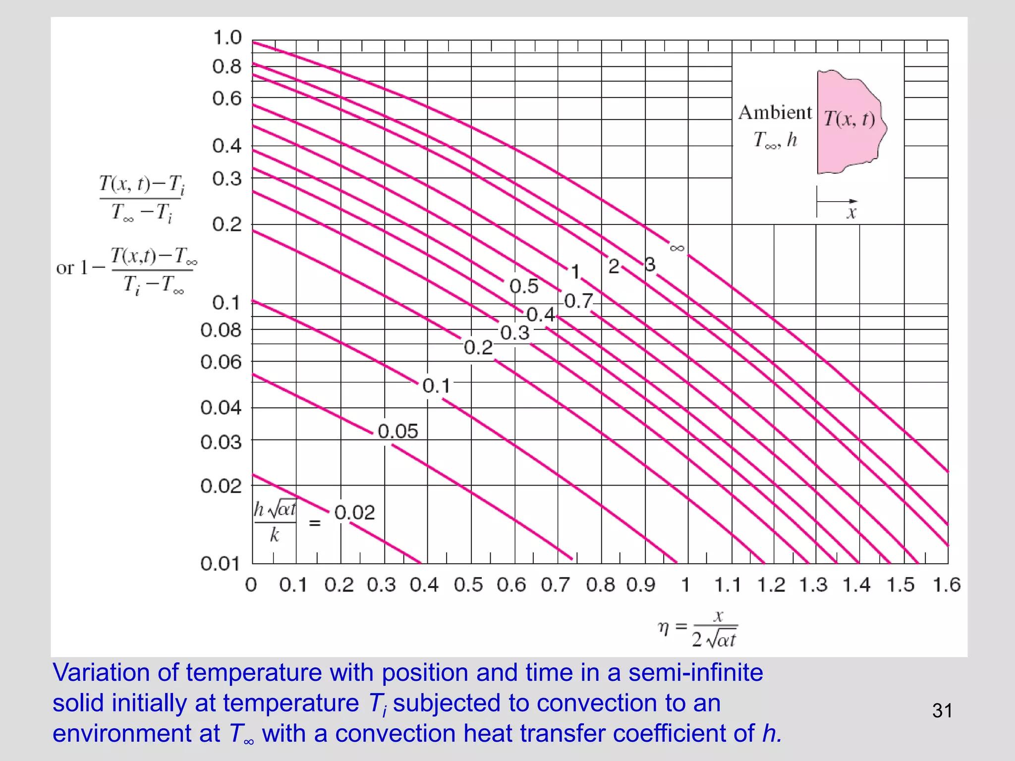
Objective: To estimate the local HTC at the surface of a vial or container during a freeze-drying cycle. Principle: For early times (Fo < 0.2), a semi-infinite solid subjected to a convective boundary condition has an analytical solution. The temperature response at a depth x is given by the complementary error function: (T(x,t)-T∞)/(Ti-T∞) = erfc[ x/(2√(αt)) ] - exp(hx/k + h²αt/k²) * erfc[ x/(2√(αt)) + h√(αt)/k ]. For a known α and measured T(x,t), h can be regressed.

Materials: (See Scientist's Toolkit) Procedure:

• Calibration: Characterize the thermal diffusivity (α) of the frozen drug product or simulant using a validated method (e.g., modified Angström method, laser flash).
• Instrumentation: Embed a fine-gauge thermocouple (TC) at a known, shallow depth (x) from the inner base of a representative vial. Ensure minimal disturbance to heat flow.
• Process Initiation: Place the instrumented vial in a controlled lyophilizer shelf pre-cooled to a set point (e.g., -40°C). The vial's initial temperature (Ti) should be uniform and higher (e.g., 0°C).
• Data Acquisition: Record the temperature at the TC location (T(x,t)) and the shelf fluid temperature (T∞) at high frequency (≥1 Hz) from the moment of shelf contact.
• Analysis Window: Use data only from the initial period where the semi-infinite assumption holds (typically until the temperature at the vial's centerline begins to change).
• Parameter Regression: Using a computational tool (Python, MATLAB), fit the recorded T(x,t) data to the 1D semi-infinite convective model, regressing for the optimal value of h. The known values are x, α, Ti, T∞.
• Validation: Repeat across multiple vials and shelf locations to map HTC distribution.

Protocol 3.2: Validating the Biot Number Regime for a Given System

Objective: To determine whether a lumped capacitance, semi-infinite, or full finite-difference model is required for accurate thermal analysis. Principle: Calculate the Biot number using independently measured or literature values. Procedure:

• Estimate Characteristic Length (Lc): For a vial, Lc = Volume / Surface Area for heat transfer. For the base, thickness may be used.
• Determine Thermal Conductivity (k): Use literature values for the vial glass (~1.0 W/(m·K)) and, crucially, for the frozen product. Measure product k if unknown (e.g., via guarded hot plate).
• Obtain a Priori h Estimate: Use literature for similar freeze-dryer conditions or a rough order-of-magnitude calculation.
• Calculate Bi: Bi = hest * Lc / k_product.
• Model Selection:
  • If Bi < 0.1: Lumped capacitance model may suffice for full vial analysis.
  • If Bi > 0.1 and analysis focuses on initial time steps: Semi-infinite model is appropriate for surface/near-surface nodes.
  • If Bi > 0.1 and analysis covers full process duration: A numerical 1D finite-difference model resolving the vial and product geometry is mandatory.

Visualizations

Title: Model Selection Workflow for HTC Determination

Title: Biot Number Regimes and Model Selection

The Scientist's Toolkit

Table 3: Essential Research Reagents & Materials for HTC Experiments

Item	Function/Specification	Application Note
Model Frozen Solution (e.g., 5% w/v Sucrose)	A well-characterized simulant for biologic formulations. Known α and k values allow method validation.	Use as a standard to calibrate experimental setup before testing novel, expensive APIs.
Fine-Gauge T-Type Thermocouples (36-40 AWG)	Minimize thermal mass and perturbation of the temperature field. Fast response time.	Calibrate against NIST-traceable standards. Ensure junction is precisely positioned at depth x.
Data Acquisition System (DAQ)	High-resolution (≥16-bit), multi-channel, with sampling rate ≥10 Hz.	Synchronize temperature readings with process events (shelf movement, pressure change).
Reference Thermal Conductivity Sensor (e.g., KD2 Pro)	Measures k of frozen or liquid materials independently.	Required for calculating α from measured thermal diffusivity or for direct Bi calculation.
Calibrated Lyophilization Vials (e.g., 6R)	Standard geometry ensures consistent characteristic length (L_c) for Bi calculation.	Pre-measure wall thickness and bottom curvature for accurate geometric modeling.
Thermal Bath & Standard Reference Material	For calibrating thermocouples at fixed points (e.g., ice-water bath at 0°C).	Essential for ensuring absolute temperature accuracy better than ±0.2°C.
Computational Software (Python w/ SciPy, MATLAB)	For non-linear regression of h from temperature data using the transcendental semi-infinite solution.	Implement error function (erfc) and robust fitting algorithms (e.g., Levenberg-Marquardt).

This document presents experimental protocols and application notes for three biomedical procedures—skin surface cooling, laser tissue interaction, and thermal probe insertion—framed within the thesis research on 1D unsteady heat conduction for semi-infinite wall Heat Transfer Coefficient (HTC) research. The core thesis investigates transient thermal boundary conditions in biological tissues, modeled as semi-infinite domains. The experimental analogs provide a practical validation framework for the theoretical models, crucial for researchers, scientists, and drug development professionals working in thermal therapies, diagnostic probe design, and transdermal delivery systems.

Application Notes & Protocols

Application Note: Skin Surface Cooling (Cryotherapy Analog)

Thesis Link: Models the transient surface heat flux and temperature gradient into the tissue (semi-infinite medium) following a sudden application of a cold boundary condition.

Protocol: Experimental Measurement of Surface HTC During Cryogen Spray Cooling

• Objective: To quantify the effective heat transfer coefficient (h) between a cryogen spray and skin phantom/human skin in vivo.
• Materials: See Scientist's Toolkit (Table 1).
• Procedure:
  • Prepare a skin phantom (agar-based with defined thermal properties) or obtain IRB approval for in vivo study.
  • Embed micro-thermocouples at depths of 50 µm, 100 µm, and 200 µm beneath the surface, or use a high-speed infrared (IR) camera for surface temp mapping.
  • Stabilize initial tissue temperature to 32°C (for in vivo) or 37°C (for phantom).
  • Activate the cryogen spray (e.g., tetrafluoroethane) for a controlled duration (e.g., 20-100 ms) at a fixed distance (30 mm).
  • Simultaneously record temperature-time (T-t) history at all sensor depths at ≥1 kHz sampling rate.
  • Post-Processing: Fit the recorded sub-surface T-t data to the analytical solution of 1D unsteady conduction in a semi-infinite solid with a convective boundary condition (Newton's law of cooling). The fitting parameter is the effective HTC (h).

Table 1: Quantitative Data from Cryogen Spray Cooling Studies

Parameter	Typical Range	Measurement Technique	Relevance to 1D Model
Spray Duration	20 – 100 ms	Solenoid valve controller	Defines the time-boundary condition
Effective HTC (h)	5,000 – 15,000 W/m²·K	Inverse solution from T-t data	Primary fitted parameter in semi-infinite model
Surface Temp Drop	20°C to -30°C	High-speed IR thermography	Validates model-predicted surface condition
Thermal Depth (δ)	100 – 500 µm	Depth of significant cooling after 100 ms	δ ≈ √(αt); key model prediction

Title: Inverse Method to Determine HTC from Cooling Data

Application Note: Laser Tissue Interaction (Photothermal Therapy Analog)

Thesis Link: Models the volumetric heat generation term (q''') from light absorption and its unsteady conduction, with surface cooling as a boundary condition to protect the epidermis.

Protocol: Combined Laser Irradiation and Dynamic Cooling for Selective Photothermolysis

• Objective: To optimize laser parameters and cooling pulse timing to achieve target damage in a dermal chromophore while preserving the epidermis.
• Materials: See Scientist's Toolkit (Table 2).
• Procedure:
  • Select laser wavelength (e.g., 755 nm for melanin, 1064 nm for deeper vessels) and pulse duration (0.5-100 ms).
  • Configure dynamic cooling device (DCD) to deliver a cryogen spurt either before (pre-), during (parallel), or after (post-) laser pulse.
  • Use tissue phantom containing target chromophore (e.g., India ink for blood) at specified depth.
  • Irradiate phantom with single laser pulse at known fluence (J/cm²). Record spatiotemporal temperature field using high-resolution IR camera or thermal imaging probe.
  • Vary DCD delay time (e.g., -10 to +50 ms relative to laser) and duration.
  • Analyze data by comparing measured temperature rise at target depth and epidermis to 1D model predictions incorporating Penne's Bioheat Equation (simplified to 1D conduction with source).

Table 2: Quantitative Data for Laser-Tissue Interaction

Parameter	Typical Range	Measurement Technique	Relevance to 1D Model
Laser Fluence	5 – 100 J/cm²	Energy meter / beam area	Input for heat source term (q''')
Optical Penetration Depth (δ_opt)	0.1 – 3 mm	Spectrophotometry on tissue	Defines exponential decay of q'''(z)
Epidermal Cooling HTC	3,000 – 10,000 W/m²·K	As per Protocol 2.1	Boundary condition for 1D model
Thermal Relaxation Time	0.1 – 10 ms	τ = δ² / (4α)	Key time constant in unsteady solution

Title: Coupled Laser Heating and Surface Cooling Model

Application Note: Thermal Probe Insertion (Thermocouple/Ablation Probe Analog)

Thesis Link: Models the transient disturbance caused by inserting a cold (or hot) probe into tissue, treating the probe as a line source/sink in a semi-infinite medium.

Protocol: Measurement of Tissue Thermal Properties via Transient Needle Probe

• Objective: To determine tissue thermal diffusivity (α) and conductivity (k) in situ by analyzing the cooling curve of a pre-heated needle probe.
• Materials: See Scientist's Toolkit (Table 3).
• Procedure:
  • Calibrate a needle thermistor probe (diameter < 1 mm) containing both a heating element and temperature sensor.
  • Insert probe into target tissue (ex vivo sample or in vivo under guidance).
  • Allow probe-tissue system to reach thermal equilibrium (T0).
  • Activate internal heater for a short period (1-5 s) to raise probe temperature by ~5-10°C.
  • Deactivate heater and record the natural cooling temperature-time data of the probe at high frequency.
  • Analyze the cooling curve by fitting it to the theoretical solution for an ideal line heat source in an infinite/semi-infinite medium. The slope of the linear region of T vs. ln(t) plot yields thermal conductivity.

Table 3: Quantitative Data for Transient Needle Probe Method

Parameter	Typical Range	Measurement Technique	Relevance to 1D Model
Probe Diameter	0.5 – 1.2 mm	Manufacturer spec	Determines applicability of line-source model
Heating Time	1 – 10 s	Controlled pulse	Must be short for transient assumption
Measured k (Soft Tissue)	0.3 – 0.6 W/m·K	Slope of T vs. ln(t) plot	Primary output from line-source solution
Measured α (Soft Tissue)	0.12 – 0.15 mm²/s	From full time-domain fit	Secondary output from model fit

Title: Thermal Property Measurement via Transient Probe

The Scientist's Toolkit: Research Reagent Solutions & Essential Materials

Table 4: Essential Materials for Featured Experiments

Item Name	Function/Brief Explanation	Example Product/Chemical
Agar-Based Tissue Phantom	Simulates optical & thermal properties of human skin for controlled, repeatable experiments.	Agar (4-6%), India ink (absorber), Intralipid (scatterer), water.
Cryogen Spray (HFC-134a)	Provides rapid, controllable convective surface cooling with high heat transfer coefficient.	Tetrafluoroethane (Genetron 134a).
High-Speed IR Camera	Non-contact, high-resolution mapping of surface temperature dynamics with millisecond resolution.	FLIR A655sc, Telops FAST M3.
Micro-Thermocouple Array	Invasive but precise measurement of subsurface temperature gradients (T(z,t)).	Type T or K thermocouples, 50µm bead diameter.
Diode Laser System	Provides controlled, monochromatic optical radiation for photothermal studies.	Crystall.aser, 755 nm or 1064 nm, pulsed operation.
Transient Needle Probe	Combined heater/sensor for in-situ measurement of thermal properties via line-source method.	Hukseflux TP08, KD2-Pro sensor.
Data Acquisition (DAQ) System	High-frequency synchronous recording of multiple temperature and control signals.	National Instruments USB-6363, >1 MS/s.
Inverse Heat Transfer Solver	Custom software (MATLAB, Python) to fit HTC & properties to analytical 1D models.	Algorithm based on Levenberg-Marquardt optimization.

From Theory to Practice: Analytical Solutions and Numerical Methods for Biomedical HTC Problems

This document details the application of the classical error function (erf) and complementary error function (erfc) to solve the 1D unsteady heat conduction equation for a semi-infinite solid. Within the broader thesis on Heat Transfer Coefficient (HTC) research for semi-infinite wall models, this analytical approach is foundational for validating experimental and numerical methods used in thermal characterization, with direct applications in materials science and drug development processes like lyophilization and controlled-release formulation stability testing.

Fundamental Analytical Solution

The governing equation for one-dimensional, unsteady heat conduction in a semi-infinite solid with constant thermal properties is: [ \frac{\partial T}{\partial t} = \alpha \frac{\partial^2 T}{\partial x^2} ] where ( T ) is temperature, ( t ) is time, ( x ) is the spatial coordinate (penetration depth), and ( \alpha ) is thermal diffusivity.

For a semi-infinite wall initially at a uniform temperature ( Ti ), subjected to a constant surface temperature ( Ts ) at ( t > 0 ), the solution is: [ \frac{T(x,t) - Ts}{Ti - Ts} = \operatorname{erf}\left( \frac{x}{2\sqrt{\alpha t}} \right) ] Equivalently, using the complementary error function: [ \frac{T(x,t) - Ti}{Ts - Ti} = \operatorname{erfc}\left( \frac{x}{2\sqrt{\alpha t}} \right) ]

The key dimensionless parameter is the similarity variable ( \eta = \frac{x}{2\sqrt{\alpha t}} ). The heat flux at the surface (( x=0 )) is given by: [ qs''(t) = -k \frac{\partial T}{\partial x}\Big|{x=0} = \frac{k (Ts - Ti)}{\sqrt{\pi \alpha t}} ] where ( k ) is thermal conductivity.

Quantitative Data and Key Relationships

Table 1: Core Properties of erf and erfc Functions

Function	Definition	Key Property	Limiting Values
Error Function (erf)	(\operatorname{erf}(z) = \frac{2}{\sqrt{\pi}} \int_0^z e^{-\eta^2} d\eta)	(\operatorname{erf}(-z) = -\operatorname{erf}(z))	(\operatorname{erf}(0)=0), (\operatorname{erf}(\infty)=1)
Complementary Error Function (erfc)	(\operatorname{erfc}(z) = 1 - \operatorname{erf}(z))	(\operatorname{erfc}(-z) = 2 - \operatorname{erfc}(z))	(\operatorname{erfc}(0)=1), (\operatorname{erfc}(\infty)=0)

Table 2: Temperature Regime and Corresponding Analytical Form

Boundary Condition at x=0	Analytical Solution	Application Context in HTC Research
Constant Temperature	(\frac{T-Ti}{Ts-T_i} = \operatorname{erfc}(\eta))	Calibration benchmark for constant-temperature baths or plates.
Constant Heat Flux	(T(x,t) = Ti + \frac{qs''}{k}[2\sqrt{\frac{\alpha t}{\pi}}e^{-\eta^2} - x \operatorname{erfc}(\eta)])	Modeling laser heating or constant-power sources.
Convective Boundary (Newtonian Cooling)	(\frac{T-Ti}{T\infty-T_i} = \operatorname{erfc}(\eta) - e^{hx/k + h^2\alpha t/k^2}\operatorname{erfc}(\eta + \frac{h\sqrt{\alpha t}}{k}))	Direct determination of HTC (h) from temperature data.

Experimental Protocol: Determining HTC via Transient Semi-Infinite Assumption

AIM: To experimentally determine the convective Heat Transfer Coefficient (h) at the surface of a material using the analytical erfc solution with a convective boundary condition.

PROTOCOL:

• Material Preparation:

  • Select a test material (e.g., polished metal slab, hydrogel block for biomimetic studies) that can be approximated as semi-infinite for the experiment's duration. This requires the material thickness ( L > 4\sqrt{\alpha t_{exp}} ).
  • Instrument the sample with a minimum of three calibrated thermocouples or resistance temperature detectors (RTDs) at known depths ( x1, x2, x_3 ) from the exposed surface.
  • Ensure the initial temperature ( T_i ) of the sample is uniform in a controlled environmental chamber.

• Experimental Procedure:

  • At time ( t=0 ), expose the material's surface to a fluid (air, liquid coolant) at a known, constant free-stream temperature ( T\infty \neq Ti ).
  • Simultaneously initiate high-frequency data acquisition (≥10 Hz) from all embedded temperature sensors.
  • Record temperature-time histories ( T(xn, t) ) until the temperature change at the deepest sensor is measurable but remains small (<5% of ( (T\infty - T_i) ) to preserve semi-infinite conditions).

• Data Analysis for HTC Extraction:

  • For a selected time ( t ), plot the measured temperature profile ( T ) vs. depth ( x ).
  • Fit the analytical solution for a convective boundary condition (Table 2) to the experimental ( T(x) ) data using non-linear regression.
  • The primary fitting parameter is the Heat Transfer Coefficient ( h ). Secondary fitted parameters can include ( \alpha ) and ( T_\infty ) for validation.
  • Repeat the fitting procedure for multiple times ( t ) during the valid experimental period. The consistency of the derived ( h ) value validates the model assumptions.

The Scientist's Toolkit: Research Reagent Solutions & Essential Materials

Table 3: Essential Materials for Experimental HTC Research

Item	Function in Experiment
High-Conductivity Calibration Block (e.g., Copper, Aluminum)	Provides a reference material with well-known thermal properties (( k, \alpha )) for method validation and sensor calibration.
Biomimetic Hydrogel or Agarose Slab	Models biological tissues or drug matrices in pharmaceutical development studies of drying or freezing processes.
Micro-encapsulated Phase Change Material (PCM)	Used to create test materials with specific, temperature-dependent thermal properties for studying complex boundary conditions.
Calibrated Thermocouple Arrays	Provide precise, spatially-resolved temperature measurement within the test specimen. Fine-wire (< 0.1mm) types minimize disturbance.
Data Acquisition System (DAQ)	High-speed, multi-channel system for synchronous logging of temperature data from all sensors.
Controlled Temperature Bath/Joule	Maintains a constant, uniform free-stream temperature (( T_\infty )) for the convective fluid.
Thermal Interface Material (TIM)	Ensures perfect thermal contact between sensors and the test material, eliminating contact resistance artifacts.
Numerical Computing Software (e.g., Python with SciPy, MATLAB)	Platform for implementing non-linear regression fits of the erf/erfc solution to experimental data and calculating derived parameters like ( h ).

Visualized Workflows and Relationships

Title: Analytical Pathway for 1D Semi-Infinite Heat Conduction Solutions

Title: Experimental Protocol to Determine Convective HTC

Application Notes

This document details the implementation and validation of the exact analytical solution for one-dimensional, unsteady heat conduction in a semi-infinite solid. This work forms a foundational component of a broader thesis on Heat Transfer Coefficient (HTC) characterization for transient thermal processes, with applications ranging from materials science to controlled-temperature drug storage and lyophilization process development.

The governing partial differential equation (PDE) is the heat diffusion equation: ∂T/∂t = α (∂²T/∂x²) where T is temperature, t is time, x is depth, and α is thermal diffusivity.

For a semi-infinite wall (x ≥ 0) with initial condition T(x,0) = Ti, and a constant surface temperature boundary condition T(0,t) = Ts for t > 0, the exact solution is given by: (T(x,t) - Ts) / (Ti - Ts) = erf( x / (2√(αt)) ) where erf is the Gauss error function.

The solution provides the temperature profile T(x,t) for any depth and time, which is critical for calibrating experimental HTC measurements and validating numerical models.

Table 1: Key Parameters in 1D Unsteady Heat Conduction

Parameter	Symbol	Unit	Typical Range (Example Materials)	Role in Solution
Thermal Diffusivity	α	m²/s	~1.5e-5 (Steel), ~1.4e-7 (Water)	Determines rate of heat penetration.
Initial Temperature	T_i	°C or K	Environment-dependent	Reference state for the solid.
Surface Temperature	T_s	°C or K	Controlled boundary condition	Drives the thermal transient.
Depth	x	m	0 to characteristic depth	Independent variable for profile.
Time	t	s	From initial application	Independent temporal variable.

Table 2: Sample Calculated Temperature Penetration (Ti = 100°C, Ts = 0°C, α = 1.0e-6 m²/s)

Time (s)	Depth where (T-Ts)/(Ti-T_s) = 0.5 (m)	Heat Penetration Depth δ (≈√(12αt)) (m)
60	0.00095	0.00268
600	0.00300	0.00849
3600	0.00735	0.02078

Experimental Protocols

Protocol 1: Validation of Exact Solution Using a Controlled Thermal Plate

Objective: To experimentally measure temperature profiles over time in a thick material and compare to the exact analytical solution, thereby validating the model assumptions (semi-infinite behavior, constant properties).

Materials & Equipment:

• Thermal Plate Apparatus with precise surface temperature control (±0.1°C).
• Test specimen block (e.g., Plexiglas, Teflon) of sufficient thickness (≥5× calculated penetration depth).
• An array of calibrated micro-thermocouples (Type T or K) or resistance temperature detectors (RTDs).
• Data acquisition system with multi-channel logging (≥1 Hz sampling rate).
• Thermal paste for ensuring minimal contact resistance.
• Insulating material to wrap sides of specimen, enforcing 1D heat flow.

Procedure:

• Specimen Preparation: Embed thermocouples at precise, known depths (e.g., 1mm, 3mm, 5mm, 10mm) from the surface to be heated. Ensure the lateral spacing is sufficient to prevent interference.
• Initialization: Place the specimen on the insulated bench. Allow it to equilibrate to a uniform initial temperature (Ti). Record Ti for all sensors.
• Boundary Condition Application: Activate the thermal plate to the target surface temperature (T_s). Immediately bring it into firm, uniform contact with the specimen surface (x=0). Start data acquisition simultaneously.
• Data Collection: Record temperatures from all embedded sensors for the duration of the experiment (until the deepest sensor shows a significant change).
• Post-Processing: For each time step t, plot the measured temperature T against depth x.
• Model Fitting: Assume an initial estimate for thermal diffusivity (α). For each (x,t) data point, calculate the dimensionless temperature θ = (T - Ts)/(Ti - T_s). Compare to the analytical solution θ = erf( x / (2√(αt)) ). Perform a least-squares regression to find the α that minimizes the error between model and data.
• Validation: Compare the fitted α with literature values. Assess the goodness-of-fit (e.g., R²) to confirm the applicability of the semi-infinite, constant-property model.

Protocol 2: Inverse Estimation of Heat Transfer Coefficient (HTC)

Objective: To use the exact solution as a forward model in an inverse algorithm to estimate the convective HTC from transient temperature measurements at a single depth.

Background: For a convective boundary condition -k ∂T/∂x = h(T_∞ - T(0,t)), an exact solution exists involving complementary error functions. A common inverse method uses temperature-time data at a single interior point (x = x₁) to find h.

Procedure:

• Experimental Setup: Similar to Protocol 1, but the specimen surface is exposed to a fluid flow (e.g., air, water) at a known bulk temperature T_∞. Use at least one accurately placed interior thermocouple at depth x₁.
• Transient Experiment: Subject the specimen initially at Ti to the convective environment at T∞. Record the temperature history T(x₁, t) at the interior location.
• Inverse Algorithm: a. Postulate a value for the HTC (h). b. Using the exact analytical solution for the convective boundary condition, calculate the predicted temperature history at depth x₁: Tcalc(x₁, t; h). c. Define an objective function, e.g., Sum( [Tmeasured(t) - T_calc(t; h)]² ). d. Use an optimization routine (e.g., Gauss-Newton, Levenberg-Marquardt) to iterate h until the objective function is minimized.
• Uncertainty Analysis: Perform a sensitivity analysis to determine the uncertainty in the estimated h based on measurement uncertainties in x₁, α, and T.

The Scientist's Toolkit

Table 3: Essential Research Reagents & Materials for HTC Studies

Item	Function & Relevance
High-Conductivity Thermal Paste	Minimizes contact resistance between heaters/coolers and test specimens, ensuring accurate boundary condition implementation.
PEEK or Teflon Specimen Blocks	Low thermal diffusivity materials extend the semi-infinite time window, making experiments more manageable.
Micro-fabricated Thin-Film Heat Flux Sensors	Directly measure heat flux at the surface (q"), providing a direct comparison to -k(∂T/∂x) from the model.
Phase-Change Materials (e.g., Gallium)	Used for creating precise isothermal boundary conditions (T_s = constant) during validation experiments.
Data Acquisition Software with Real-Time FFT	Enables monitoring of thermal response in frequency domain, useful for validating linearity of the system.
Certified Reference Material (CRM) for Thermal Diffusivity (e.g., NIST SRM 8420 series)	Provides an absolute standard for calibrating the entire measurement chain and validating the fitted α.

Visualizations

Derivation of Exact Solution for Constant Surface Temperature

Workflow for Validating the Exact Solution Experimentally

Inverse Method for HTC Estimation from Temperature Data

Conceptual Framework & Mathematical Formulation

The 1D unsteady heat conduction equation for a semi-infinite solid (x ≥ 0) is given by the parabolic partial differential equation (PDE):

∂T/∂t = α (∂²T/∂x²) for 0 ≤ x < ∞, t > 0

where:

• T: Temperature (K)
• t: Time (s)
• x: Spatial coordinate from the surface (m)
• α: Thermal diffusivity (m²/s), α = k / (ρ c_p)

Common initial and boundary conditions relevant to HTC (Heat Transfer Coefficient) research include:

• Initial Condition (IC): T(x,0) = T_initial
• Boundary Condition at x=0 (Surface): -k ∂T/∂x|{x=0} = h (Tfluid - T_surface) (Convective/Robin condition)
• Boundary Condition as x→∞: T(∞,t) = T_initial (Dirichlet condition)

Discretization Strategy for a Semi-Infinite Domain

The core challenge is simulating an infinite domain on a finite computational grid. The primary strategy is the use of a coordinate transformation or a truncated domain with an artificial boundary condition.

Domain Truncation and Artificial Boundary

The semi-infinite domain is approximated by a finite domain of length L, where L is chosen such that the thermal penetration depth δ(t) << L for the duration of the simulation.

Parameter	Symbol	Typical Range/Value	Justification
Computational Domain Length	L	≥ 10√(α t_max)	Ensures negligible temperature change at x=L for final time t_max.
Thermal Diffusivity (Water)	α	~1.43 x 10⁻⁷ m²/s	Used for calibration in bio-heat transfer contexts.
Penetration Depth Estimate	δ(t)	~√(4α t)	Depth where significant temperature change occurs.
Grid Points (Spatial)	N	100 - 500	Balances accuracy and computational cost.
Time Steps	M	Variable (CFL dependent)	Determined by stability criteria.

Finite Difference Discretization Schemes

Common FDM schemes are applied to the internal nodes of the discretized 1D grid.

Scheme	Finite Difference Formulation (Internal Node i)	Stability Condition (Explicit)	Order of Accuracy
Forward Time Central Space (FTCS) - Explicit	(Ti^{n+1} - Ti^n)/Δt = α (T{i-1}^n - 2Ti^n + T_{i+1}^n)/Δx²	αΔt/Δx² ≤ 0.5	O(Δt, Δx²)
Crank-Nicolson - Implicit	(Ti^{n+1} - Ti^n)/Δt = (α/2)[(∂²T/∂x²)^ni + (∂²T/∂x²)^{n+1}i]	Unconditionally Stable	O(Δt², Δx²)
Fully Implicit	(Ti^{n+1} - Ti^n)/Δt = α (T{i-1}^{n+1} - 2Ti^{n+1} + T_{i+1}^{n+1})/Δx²	Unconditionally Stable	O(Δt, Δx²)

Boundary Condition Implementation

The convective boundary condition at x=0 is discretized using a ghost node or a finite difference approximation.

Boundary	Condition Type	Discretization (FTCS Example)	Implementation Notes
Surface (x=0)	Convective (Robin)	-k (T1^n - T{-1}^n)/(2Δx) ≈ h (Tfluid - T0^n) Eliminates ghost node T_{-1}	Results in a modified equation for T0^{n+1} linking T0^n and T_1^n.
Truncated Edge (x=L)	Adiabatic (Neumann) or Constant Temperature	Adiabatic: ∂T/∂x = 0 → T{N+1}^n = T{N-1}^n Constant: TN^n = Tinitial	Adiabatic is common if L is sufficiently large. Constant is simpler but less accurate if L is not large enough.

Experimental Protocol: Numerical HTC Estimation

This protocol outlines the steps to estimate the Heat Transfer Coefficient (h) by matching a numerical FDM solution to experimental temperature data.

Objective: To determine the unknown convective HTC (h) at the surface of a semi-infinite solid by minimizing the error between simulated and measured temperature-time histories at an embedded sensor location.

Step 1 – Problem Setup & Discretization

• Define material properties (k, ρ, c_p) of the test medium.
• Specify the initial temperature (Tinitial) and the fluid temperature (Tfluid).
• Truncate the domain at length L (e.g., L = 10√(α t_total)).
• Discretize space (choose N, calculate Δx) and time (choose M, calculate Δt respecting CFL if using explicit scheme).

Step 2 – Implement Numerical Solver

• Code the selected FDM scheme (e.g., Implicit for stability).
• Implement the discretized convective boundary condition at x=0.
• Implement the chosen artificial boundary condition at x=L (e.g., adiabatic).
• Validate the solver with a known analytical solution (e.g., sudden change in surface temperature).

Step 3 – Inverse Parameter Estimation

• Input: Obtain experimental temperature vs. time data, Texp(t), at a known depth xsensor.
• Initial Guess: Provide an initial estimate for h (e.g., 100 W/m²K for air, 1000 W/m²K for water).
• Forward Run: Execute the FDM solver using the current guess for h.
• Error Calculation: Compute the root-mean-square error (RMSE) between the simulated Tsim(xsensor, t) and T_exp(t).
• Optimization: Use an iterative optimization algorithm (e.g., Golden-section search, Gauss-Newton) to adjust h to minimize the RMSE.
• Output: The value of h that yields the best fit between the model and experimental data.

Visualization of the FDM Workflow

Title: Finite Difference Method Workflow for 1D Heat Conduction

Title: Inverse Protocol for HTC Estimation Using FDM

The Scientist's Toolkit: Research Reagent Solutions

Item/Category	Function in Numerical HTC Research	Example/Specification
Computational Core	Executes the FDM solver and optimization routines.	MATLAB/Python (NumPy, SciPy), Julia, or C/Fortran. High-performance computing cluster for large parameter sweeps.
Numerical ODE/PDE Library	Provides tested, efficient solvers and optimization tools.	SciPy's integrate and optimize modules, MATLAB's PDE Toolbox, FiPy (Python).
Experimental Calibration Data	Ground truth temperature profiles for inverse estimation.	Thermocouple or infrared camera data measuring T(t) at known depths within a material sample.
Material Property Database	Provides accurate thermal properties (k, ρ, c_p) for the simulated medium.	NIST databases, published material property tables for tissues, polymers, or construction materials.
Mesh Generation Tool	Creates the spatial discretization grid.	Custom scripts for 1D uniform grids. Tools like Gmsh for complex 2D/3D extensions.
Visualization & Analysis Suite	Post-processes results, compares simulation to data, creates plots.	Matplotlib, ParaView, Tecplot, OriginLab.
Validation Benchmark	Analytical solution used to verify the FDM implementation.	Exact solution for T(x,t) in a semi-infinite solid with a constant surface temperature change.

This protocol details the construction of a simple Explicit Finite Difference Method (FDM) solver for 1D unsteady heat conduction. The work is framed within a broader thesis investigating Heat Transfer Coefficients (HTC) at the boundary of a semi-infinite solid, a problem relevant to biomedical applications such as localized hyperthermia in drug delivery or thermal analysis of tissue.

Core Mathematical Model

The governing partial differential equation (PDE) for 1D unsteady heat conduction is the Fourier equation: [ \frac{\partial T}{\partial t} = \alpha \frac{\partial^2 T}{\partial x^2} ] where ( T ) is temperature, ( t ) is time, ( x ) is spatial coordinate, and ( \alpha ) is thermal diffusivity.

For a semi-infinite wall ((0 \leq x < \infty)) with a convective boundary condition at (x=0): [ -k \frac{\partial T}{\partial x}\bigg|{x=0} = h \left( T\infty - T(0,t) \right) ] where ( k ) is thermal conductivity, ( h ) is the convective heat transfer coefficient (HTC), and ( T_\infty ) is the ambient fluid temperature.

Finite Difference Discretization (Explicit Scheme)

Domain Discretization

The spatial domain is truncated at a sufficient depth ( L ) and discretized into ( N ) nodes.

• Spatial step: ( \Delta x = L / (N-1) )
• Time step: ( \Delta t )

Stability Criterion (Von Neumann)

The explicit method is conditionally stable. The stability requirement is: [ \text{Fo} = \frac{\alpha \Delta t}{(\Delta x)^2} \leq \frac{1}{2} ] where Fo is the grid Fourier number.

Finite Difference Equations

• Interior Nodes (i = 2 to N-1): [ Ti^{\text{new}} = Ti^{\text{old}} + \text{Fo} \cdot (T{i+1}^{\text{old}} - 2Ti^{\text{old}} + T_{i-1}^{\text{old}}) ]
• Convective Boundary Node (i = 1): Using a forward difference for the gradient. [ T1^{\text{new}} = T1^{\text{old}} + \text{Fo} \cdot \left[ 2T2^{\text{old}} - 2T1^{\text{old}} - \frac{2h\Delta x}{k} (T1^{\text{old}} - T\infty) \right] ]
• Deep Boundary Node (i = N): Assumed adiabatic or constant initial temperature (( \partial T/\partial x = 0 )). [ TN^{\text{new}} = TN^{\text{old}} + \text{Fo} \cdot (2T{N-1}^{\text{old}} - 2TN^{\text{old}}) ]

Quantitative Parameters for Benchmarking

Table 1: Standard Material and Numerical Parameters

Parameter	Symbol	Value	Unit	Purpose in Simulation
Thermal Conductivity	( k )	0.5	W/m·K	Tissue-like material property
Thermal Diffusivity	( \alpha )	1.5e-7	m²/s	Controls rate of heat diffusion
Heat Transfer Coeff. (Low)	( h_{\text{low}} )	10	W/m²·K	Simulates natural convection
Heat Transfer Coeff. (High)	( h_{\text{high}} )	1000	W/m²·K	Simulates forced convection/cooling
Ambient Temperature	( T_\infty )	20	°C	Driving fluid temperature
Initial Wall Temperature	( T_{\text{init}} )	100	°C	Initial condition
Wall Depth (Simulated)	( L )	0.1	m	Truncated semi-infinite domain
Spatial Nodes	( N )	51	-	Resolution of spatial grid
Simulation Time	( t_{\text{final}} )	10,000	s	Total simulated physical time

Table 2: Impact of Discretization on Stability & Runtime

(\Delta x) (m)	Max Stable (\Delta t) (s) (Fo=0.5)	Total Time Steps for 10,000s	Relative Runtime (Arb. Units)
0.010	333.3	30	1.0 (Baseline)
0.005	83.3	120	4.0
0.002	13.3	752	25.1

Step-by-Step Implementation Protocol

Python Implementation Code

MATLAB Implementation Code

Validation & Analysis Protocol

• Stability Verification: Run the solver with Fo = 0.5, 0.51, and 0.6. Observe unstable, oscillatory solutions when the criterion is violated.
• HTC Sensitivity Analysis: Execute the solver with the low (10 W/m²·K) and high (1000 W/m²·K) HTC values from Table 1. Compare the cooling rate at the surface (x=0).
• Grid Independence Test: Run simulations for N = 26, 51, and 101. Compare the temperature profile at t = 5000s. The results for N=51 and N=101 should be nearly identical.
• Comparison with Analytical Solution (Optional): For a constant surface temperature boundary condition (Dirichlet), compare the numerical result with the analytical error function solution.

The Scientist's Toolkit: Research Reagent Solutions

Table 3: Essential Computational & Analytical Materials

Item	Function in HTC Research
Explicit FDM Solver	Core algorithm for simulating transient temperature fields.
Parameter Sweep Script	Automates simulation across a range of HTC, (k), or (\alpha) values.
Sensitivity Analysis Module	Quantifies the influence of input parameter uncertainty on the predicted temperature.
Data Fitting Tool (e.g., curve_fit)	Used to inversely estimate the HTC from experimental temperature data by minimizing the difference between solver output and measurement.
Visualization Suite	Generates 2D/3D plots of temperature profiles, heat flux, and convergence history.

Process and Logical Relationship Diagrams

Title: Explicit FDM Solver Workflow for 1D Heat Conduction

Title: Inverse Estimation of HTC from Experimental Data

The analysis of 1D unsteady heat conduction in a semi-infinite solid is fundamental for modeling transient thermal interactions at biological interfaces. This thesis chapter applies this core theory to two critical biomedical applications: the rapid freezing of skin lesions (cryotherapy) and the controlled heating of subcutaneous tissues (hyperthermia). Both cases involve a time-dependent thermal flux at the skin surface (modeled as the semi-infinite wall boundary), where the estimation of the effective Heat Transfer Coefficient (HTC) is paramount. The HTC encapsulates the complex biophysical interaction between the applied thermal device and the heterogeneous, living tissue, governing the lesion destruction depth or the therapeutic temperature zone.

Application Note: Cryotherapy for Skin Lesion Treatment

2.1. Core Principle & Modeling Objective Cryotherapy utilizes extreme cold (via liquid nitrogen spray or cryoprobe) to induce controlled cellular necrosis in lesions like warts, actinic keratosis, and superficial carcinomas. The 1D model aims to predict the spatiotemporal temperature field T(x,t) and, crucially, the penetration depth of the lethal isotherm (e.g., -40°C for many cell types) as a function of application time and surface HTC.

2.2. Key Quantitative Parameters Table 1: Key Parameters for Cryotherapy Modeling

Parameter	Symbol	Typical Value / Range	Notes
Cryogen Boiling Point	T_surf	-196°C (LN₂)	Surface boundary condition.
Lethal Tissue Temp.	T_lethal	-40°C to -50°C	Target isotherm for necrosis.
Healthy Skin Temp.	T_init	37°C	Initial condition (core).
Tissue Thermal Diffusivity	α	~1.3 x 10⁻⁷ m²/s	Varies with water/ice phase.
Effective HTC (Spray)	h	50 - 2000 W/m²K	Highly dependent on technique & device.
Treatment Time	t_tx	5 - 30 seconds	For superficial lesions.

2.3. Experimental Protocol: Ex Vivo Bovine Liver Cryotherapy Validation

Objective: To calibrate the effective HTC (h) in the 1D unsteady conduction model by matching simulated temperature profiles with experimental data from a controlled cryospray application.

Materials & Workflow:

• Sample Preparation: Prepare uniform slices of fresh bovine liver (thickness > 30mm) to approximate semi-infinite geometry. Insert fine-gauge thermocouples at depths: 1mm, 2mm, 3mm, 5mm, 7mm from the surface.
• Baseline Measurement: Record initial temperature (T_init).
• Cryogen Application: Using a standardized dermatological cryospray device, apply liquid nitrogen to the surface at a fixed distance (e.g., 10mm) and angle (90°) for a precise duration (t_tx).
• Data Acquisition: Record temperature-time histories at all thermocouple locations during and for 60 seconds post-application.
• Model Fitting: Input T_surf and T_init into the 1D unsteady conduction analytical solution. Iteratively adjust the h parameter in the convective boundary condition until the simulated T(x,t) curves best-fit the experimental thermocouple data (minimizing RMS error).
• Validation: Use the fitted h to predict the depth of the -40°C isotherm over time and compare to histological analysis of the necrotic zone in post-experiment samples.

Application Note: Controlled Microwave Hyperthermia

3.1. Core Principle & Modeling Objective Controlled hyperthermia aims to raise tissue temperature to 41-45°C for a sustained period (minutes) to sensitive cancer cells to radiation/chemotherapy or ablate them directly. A 1D model helps plan the microwave antenna power and exposure time to maintain a therapeutic temperature band within the target depth while sparing deeper healthy tissue.

3.2. Key Quantitative Parameters Table 2: Key Parameters for Hyperthermia Modeling

Parameter	Symbol	Typical Value / Range	Notes
Target Temp. Range	T_tx	41 - 45°C	Therapeutic window.
Skin Surface Temp.	T_surf	< 43°C	To avoid burn injury.
Antenna Power Density	q	10⁴ - 10⁵ W/m²	Volumetric heat source Q in Pennes' bioheat eq.
Tissue Perfusion Rate	ω_b	0.5 - 5.0 kg/m³/s	Dominant heat sink in living tissue.
Effective HTC (Cooling Pad)	h	100 - 500 W/m²K	For surface cooling devices.
Treatment Duration	t_tx	10 - 60 minutes	For deep-seated heating.

3.3. Experimental Protocol: In Vivo Murine Model Hyperthermia with Surface Cooling

Objective: To demonstrate the use of a surface cooling pad (characterized by HTC, h) to shift the peak therapeutic temperature deeper into the tissue while protecting the skin.

Materials & Workflow:

• Animal Model & Instrumentation: Anesthetize mouse with a subcutaneous tumor model. Insert micro-thermocouples at skin surface, tumor center, and deep margin. Apply a temperature-controlled cooling pad to the skin over the tumor.
• Cooling Pad Calibration: Set pad to a constant temperature (e.g., 10°C). Measure steady-state heat flux and skin temperature to calculate pad h prior to microwave activation.
• Hyperthermia Treatment: Activate planar microwave antenna at a defined power level. Simultaneously, run the cooling pad.
• Monitoring: Continuously record temperatures at all points for the treatment duration (t_tx).
• Model Simulation & Comparison: Solve the 1D Pennes' bioheat equation (extending basic conduction) incorporating the microwave source term Q and the convective boundary condition defined by the pad's h. Compare predicted temperature-depth profiles at key times with experimental measurements to validate the model's predictive power for treatment planning.

The Scientist's Toolkit

Table 3: Essential Research Reagent Solutions & Materials

Item	Function in Experiment
Liquid Nitrogen (Cryogen)	Provides extreme cold surface boundary condition for cryotherapy modeling.
Controlled-Temperature Cooling Peltier Pad	Creates a calibrated convective boundary (definable HTC) for hyperthermia skin protection.
Fine-Gauge T-Type Thermocouples (≤ 0.5mm)	Provide high-temporal-resolution temperature measurement at discrete spatial points for model validation.
Thermally Homogeneous Tissue Phantom (Agar/Gelatin)	Provides a reproducible, non-perfused medium for initial model calibration and device testing.
Infrared Thermal Camera	Provides 2D surface temperature mapping to validate boundary condition uniformity.
Programmable Microwave/RF Heat Source	Delivers precise volumetric heating for hyperthermia studies.
Data Acquisition (DAQ) System with High Sampling Rate	Synchronously logs multi-channel temperature data for transient analysis.

Visualization Diagrams

Title: Decision Flow for Thermal Therapy Modeling

Title: Cryotherapy HTC Calibration Experimental Workflow

Solving Common Challenges: Accuracy, Stability, and Efficiency in Semi-Infinite HTC Simulations

In the context of 1D unsteady heat conduction research for semi-infinite wall HTC (Heat Transfer Coefficient) characterization, a fundamental paradox arises: the physical domain extends to infinity, while computational resources are finite. The core task is to truncate this semi-infinite domain at a depth L_trunc that is computationally efficient yet introduces negligible error relative to the true semi-infinite solution. The error is governed by the propagation of the thermal penetration depth, δ(t), over the simulation time of interest.

The appropriate truncation depth depends on the material's thermal diffusivity (α), the total simulation time (t_final), and the acceptable error tolerance. The following table summarizes key quantitative criteria derived from analytical solutions to the 1D unsteady heat conduction equation.

Table 1: Truncation Depth Criteria for Semi-Infinite Domains

Criterion Name	Formula	Typical Value (Example: Steel, α=1e-5 m²/s, t_final=1000s)	Rationale & Error Bound
Thermal Penetration Depth	δ(t) ≈ √(4αt)	√(4 * 1e-5 * 1000) ≈ 0.2 m	Depth at which temperature change is ~1% of surface change. A common initial estimate.
Fixed Multiple of δ	L_trunc = N * √(4α t_final)	N=3 → L_trunc ≈ 0.6 m	Ensures boundary at x=L_trunc is essentially unperturbed. For N=3, error < 0.1%.
Error-Function-Based	L_trunc s.t. erfc(L_trunc/√(4α t_final)) < ε	For ε=1e-5, L_trunc ≈ 3.5*√(α t_final) ≈ 0.35 m	Directly links truncation depth to max error in BC satisfaction.
Numerical Stability (Explicit FD)	L_trunc must fit nodes, given Fo = αΔt/Δx² ≤ 0.5	For Δx=0.005m, nodes = 0.6/0.005 = 120	Independent criterion to ensure solution stability once domain is sized.

Table 2: Impact of Truncation Depth on Computational Cost & Error

Truncation Depth (L)	Number of Grid Nodes (Δx=0.005m)	Estimated Error at x=L (ε)	Relative Computational Cost (CPU Time)
0.2 m (1δ)	40	~1%	Baseline (1.0x)
0.4 m (2δ)	80	~0.01%	~2.0x
0.6 m (3δ)	120	~0.001%	~3.0x
1.0 m (5δ)	200	Negligible (1e-10)	~5.0x

Experimental Protocols for Validation

Protocol 3.1: Numerical Verification of Truncation Depth

Objective: To empirically determine the minimum L_trunc that yields a solution indistinguishable from a reference "near-infinite" solution.

Materials: Computational software (e.g., MATLAB, Python with NumPy), hardware meeting specifications in Table 4.

Procedure:

• Define Problem: Specify thermal diffusivity (α), surface boundary condition (e.g., step flux or convective cooling with HTC h), and total time t_final.
• Generate Reference Solution: Compute an analytical solution (e.g., using erfc) or a numerical solution on a domain much larger than 5√(4α t_final). This is the "truth" benchmark.
• Iterative Truncation Test: a. Set an initial L_trunc = √(4α t_final). b. Discretize the domain [0, L_trunc] with a sufficiently fine grid (Δx). c. Apply the surface BC and an adiabatic (∂T/∂x=0) or constant-temperature BC at x=L_trunc. d. Solve the 1D transient heat equation using a Finite Difference (e.g., Crank-Nicolson) or Finite Element method. e. Compare the simulated temperature history at a point near the surface (e.g., x=0) and at mid-domain to the reference solution. Calculate the root-mean-square error (RMSE).
• Increase L_trunc incrementally (e.g., by 0.5δ) and repeat Step 3 until the RMSE falls below a predefined threshold (e.g., 0.1% of the total temperature change).
• Document the final L_trunc as the sufficient depth for the given (α, t_final, BC) combination.

Protocol 3.2: Experimental Calibration Using a Thick Specimen

Objective: To validate the numerical model and chosen truncation depth against physical experimental data.

Procedure:

• Fabricate a "Semi-Infinite" Specimen: Use a material block (e.g., steel, polymer) with physical thickness L_phys >> √(4α t_final). Instrument with thermocouples at known depths (x1, x2, ...) from the heated/cooled surface.
• Apply Controlled Thermal Perturbation: Subject the surface to a known heat flux (via laser, heater) or convective cooling (via controlled fluid jet).
• Data Acquisition: Record temperature vs. time (T(x_i, t)) for all sensor locations throughout t_final.
• Numerical Simulation: Run a simulation matching the experimental conditions, using the candidate L_trunc and an adiabatic BC at the computational boundary.
• Inverse Estimation: Use the experimental data in an inverse algorithm (e.g., Levenberg-Marquardt) to estimate the HTC and thermal properties.
• Validation: Compare the simulated temperature profiles (using estimated parameters) directly to the experimental data. Agreement confirms the adequacy of the truncation depth and model assumptions.

Visualization of Methodology and Decision Pathway

Truncation Depth Selection & Validation Workflow

The Scientist's Toolkit: Research Reagent Solutions

Table 3: Essential Materials & Computational Tools for Semi-Infinite HTC Research

Item Name	Category	Function & Relevance
High-Thermal Effusivity Test Specimens (e.g., Stainless Steel 316, Borosilicate Glass)	Physical Material	Provides a near-ideal semi-infinite medium for experimental calibration due to low α and high rigidity.
Micro-thermocouples (T-Type, K-Type) or Infrared Thermography	Sensor	For precise, non-invasive measurement of subsurface or surface temperature history T(x,t).
Controlled Heat Flux Source (e.g., Diode Laser, Peltier Element)	Experimental Apparatus	Applies a precise, reproducible surface boundary condition (constant flux or temperature step).
Computational Software Suite (Python: NumPy/SciPy; MATLAB with PDE Toolbox; COMSOL Multiphysics)	Software	Implements finite-difference/element models, inverse algorithms, and error analysis.
High-Performance Computing Node (Multi-core CPU, ≥16GB RAM)	Hardware	Enables rapid iteration of forward simulations and parameter estimation in inverse problems.
Inverse Problem Solver (e.g., Levenberg-Marquardt, Conjugate Gradient implementation)	Algorithm	Core tool for extracting HTC and thermal properties from experimental T(x,t) data.
Dimensionless Parameter Calculator (Script for Fo, Bi, ξ)	Analysis Tool	Facilitates scaling and generalization of results from specific experiments.

This application note, framed within a broader thesis investigating 1D unsteady heat conduction for semi-infinite wall heat transfer coefficient (HTC) research, details the critical considerations for numerical stability in solving partial differential equations (PDEs). Accurate temporal simulation of temperature profiles is paramount for applications such as pharmaceutical lyophilization, sterilization process validation, and drug formulation stability testing. The note contrasts the explicit and implicit finite difference methods, focusing on the Courant-Friedrichs-Lewy (CFL) condition as a stability criterion for explicit schemes.

Foundational Theory: 1D Unsteady Heat Conduction

The governing PDE for one-dimensional, unsteady heat conduction without internal heat generation is: [ \frac{\partial T}{\partial t} = \alpha \frac{\partial^2 T}{\partial x^2} ] where ( T ) is temperature, ( t ) is time, ( x ) is spatial coordinate, and ( \alpha ) is thermal diffusivity (( \alpha = k / \rho c_p )).

Numerical Discretization: Explicit vs. Implicit Schemes

Explicit (Forward Euler) Scheme

The spatial derivative is evaluated at the current time level ( n ). [ \frac{Ti^{n+1} - Ti^n}{\Delta t} = \alpha \frac{T{i+1}^n - 2Ti^n + T{i-1}^n}{(\Delta x)^2} ] The future temperature ( Ti^{n+1} ) is solved explicitly: [ Ti^{n+1} = Ti^n + \text{Fo} \left( T{i+1}^n - 2Ti^n + T_{i-1}^n \right) ] where ( \text{Fo} = \alpha \Delta t / (\Delta x)^2 ) is the grid Fourier number.

Implicit (Backward Euler) Scheme

The spatial derivative is evaluated at the future time level ( n+1 ). [ \frac{Ti^{n+1} - Ti^n}{\Delta t} = \alpha \frac{T{i+1}^{n+1} - 2Ti^{n+1} + T{i-1}^{n+1}}{(\Delta x)^2} ] This requires solving a system of linear equations at each time step: [ -\text{Fo} \cdot T{i-1}^{n+1} + (1+2\text{Fo}) Ti^{n+1} - \text{Fo} \cdot T{i+1}^{n+1} = T_i^n ]

CFL Condition for Stability

For the explicit scheme to be numerically stable, the CFL condition (here, a stability criterion on the Fourier number) must be satisfied: [ \text{Fo} = \alpha \frac{\Delta t}{(\Delta x)^2} \leq \frac{1}{2} ] This imposes a strict limit on the time step size ( \Delta t ) relative to the spatial discretization ( \Delta x ). The implicit scheme is unconditionally stable for all ( \text{Fo} > 0 ), allowing for larger time steps at the cost of computational complexity per step.

Quantitative Comparison of Schemes

Table 1: Comparison of Explicit and Implicit Finite Difference Schemes for 1D Heat Equation

Feature	Explicit (FTCS) Scheme	Implicit (BTCS) Scheme
Stability Criterion	Conditional: ( \text{Fo} \leq 0.5 )	Unconditionally Stable
Time Step Constraint	Stringent: ( \Delta t \leq (\Delta x)^2 / (2\alpha) )	Flexible, chosen based on accuracy, not stability.
Computational Cost per Step	Low (explicit formula).	High (requires solving a tridiagonal linear system).
Algorithmic Complexity	Simple, straightforward to code.	More complex, requires solver (e.g., Thomas Algorithm).
Best Application Context	Rapid prototyping, problems with very small natural time scales or fine mesh.	Problems requiring large time steps, long simulation times, or coarse spatial grids.
Memory Requirement	Low (stores only current time level).	Moderate (must assemble matrix/right-hand side).

Table 2: Illustrative Time Step Constraints ((\alpha = 1.5 \times 10^{-7} m^2/s), Typical for Brick)

Spatial Discretization (\Delta x)	Max Stable (\Delta t) (Explicit)	Example (\Delta t) (Implicit, for Accuracy)
1.0 mm (0.001 m)	3.33 seconds	30 - 60 seconds
0.1 mm (0.0001 m)	0.0333 seconds	1 - 5 seconds
1.0 cm (0.01 m)	333.3 seconds	600 - 1800 seconds

Experimental & Numerical Protocols

Protocol 1: Implementing an Explicit Solver with CFL Check

Objective: To solve 1D transient heat conduction in a semi-infinite wall with a Dirichlet boundary condition.

• Define Parameters: Set wall properties ((k, \rho, cp)), calculate (\alpha). Define total simulation time (t{total}).
• Discretize: Choose spatial step (\Delta x) for a sufficiently thick wall (approximating semi-infinite). Calculate maximum stable time step: (\Delta t_{max} = 0.5 \cdot (\Delta x)^2 / \alpha).
• Select Time Step: Choose a practical (\Delta t \leq \Delta t_{max}). Calculate actual (\text{Fo}).
• Initialize: Set initial temperature field (T_i^0) for all spatial nodes (i).
• Apply Boundary Conditions: Set (T0^n = T{surface}) at each time step (n). For the far-field boundary (node (N)), use (TN^n = T{initial}).
• Time Marching Loop: a. For each interior node (i = 1) to (N-1), compute: (Ti^{n+1} = Ti^n + \text{Fo} \cdot (T{i+1}^n - 2Ti^n + T_{i-1}^n)). b. Update boundary conditions for time level (n+1). c. Advance time: (t = t + \Delta t).
• Terminate: Stop when (t \geq t_{total}).

Protocol 2: Implementing an Implicit Solver (Thomas Algorithm)

Objective: To solve the same problem without a CFL stability constraint.

• Steps 1-4: Same as Protocol 1.
• Select Time Step: Choose (\Delta t) based on desired temporal accuracy, independent of (\Delta x).
• Construct Linear System: For each interior node (i), form the equation: (ai T{i-1}^{n+1} + bi Ti^{n+1} + ci T{i+1}^{n+1} = di), where (ai = ci = -\text{Fo}), (bi = (1+2\text{Fo})), (di = Ti^n). Incorporate boundary conditions into coefficients for (i=1) and (i=N-1).
• Solve Tridiagonal System using the Thomas Algorithm: a. Forward Sweep: Calculate modified coefficients for (i = 1) to (N-1). b. Backward Substitution: Obtain (T_i^{n+1}) from (i = N-1) down to (1).
• Time Marching Loop: Repeat step 4 for each time step until (t \geq t_{total}).

Protocol 3: Experimental HTC Estimation via Inverse Method

Objective: To estimate the surface HTC by matching numerical model output to experimental thermal sensor data.

• Instrumentation: Embed high-precision thermocouples (e.g., T-type, uncertainty ±0.5°C) at known depths ((x1, x2)) within a test material wall.
• Experimental Run: Subject the wall surface to a thermal process (e.g., heating/cooling jet). Record temperature histories (T{exp}(xj, t)).
• Numerical Simulation: Implement an implicit solver (for stability with arbitrary (\Delta t)) in a parameter estimation loop.
• Inverse Algorithm: a. Propose an initial guess for HTC ((h)). b. Run the numerical model (Protocol 2) using this (h) as a convective boundary condition: (-k \frac{\partial T}{\partial x}\big|{x=0} = h (T{fluid} - T_{surface})). c. Compute the sum of squared errors (SSE) between simulated and experimental temperatures at sensor locations. d. Use an optimization routine (e.g., Gauss-Newton, Levenberg-Marquardt) to adjust (h) to minimize SSE. e. Iterate until convergence (e.g., relative change in (h) < 1% or SSE below tolerance).

Visualizations

Diagram 1: Numerical Scheme Decision Pathway

Diagram 2: Inverse HTC Estimation Workflow

The Scientist's Toolkit: Research Reagent Solutions & Essential Materials

Table 3: Essential Materials for 1D Unsteady HTC Research

Item / Reagent	Specification / Function
High-Conductivity Thermal Paste	Ensures minimal contact resistance between embedded sensors and host material, critical for accurate temperature measurement.
T-Type or K-Type Thermocouples	Fine-gauge (e.g., 36 AWG) for fast response time and minimal spatial disruption. Calibrated traceably for valid data.
Data Acquisition System (DAQ)	High-resolution (16-bit+), multi-channel system with cold-junction compensation and sampling rate ≥10x characteristic frequency of process.
Reference Test Material	A material with well-characterized, stable thermal properties (e.g., Polymethylmethacrylate or Austenitic Stainless Steel) for method validation.
Implicit Solver Software	Code implementing the Thomas Algorithm (in Python, MATLAB, C++, etc.) or access to validated PDE solver libraries (e.g., FiPy, MATLAB PDE Toolbox).
Optimization Suite	Software/library for nonlinear least squares (e.g., scipy.optimize.curve_fit, lsqnonlin in MATLAB) for inverse HTC estimation.
Semi-Infinite Wall Analogue	A thick slab of test material where penetration depth of thermal front is << slab thickness during experiment duration.

Optimizing Mesh and Space Step Selection for Balance Between Speed and Precision

This document provides application notes and protocols for optimizing spatial discretization (mesh and space step, Δx) and temporal discretization (time-step, Δt) in the numerical simulation of 1D unsteady heat conduction. The primary context is a doctoral thesis investigating the estimation of Heat Transfer Coefficients (HTC) for semi-infinite wall geometries, a problem relevant to thermal analysis in pharmaceutical processes (e.g., lyophilization, spray congealing) and materials science. The core challenge is balancing computational speed against numerical precision and stability to enable efficient, accurate parameter estimation (e.g., HTC) from experimental temperature data.

The explicit finite difference method is commonly employed for its simplicity. Its stability and accuracy are governed by the Fourier mesh number (Fo_m), also known as the grid Fourier number.

Key Relationship: [ Fo_m = \frac{\alpha \Delta t}{(\Delta x)^2} ] Where α is thermal diffusivity.

For stability in a 1D explicit scheme, the criterion is Fo_m ≤ 0.5. Precision is improved by reducing both Δx and Δt, but at a nonlinear computational cost.

Table 1: Impact of Discretization Parameters on Simulation Metrics

Parameter Change	Computational Speed	Numerical Precision (Truncation Error)	Stability (Explicit Method)	Recommended For
Increase Δx (coarser mesh)	Increases (fewer nodes)	Decreases (O(Δx²) error)	Improves (lowers Fom)	Initial scoping, low-gradient regions
Decrease Δx (finer mesh)	Decreases (more nodes)	Increases (O(Δx²) error)	Challenges (raises Fom)	Capturing steep gradients (near surface)
Increase Δt	Increases (fewer iterations)	Decreases (O(Δt) error)	Risk of Instability (raises Fom)	Stable, slow-transient regimes
Decrease Δt	Decreases (more iterations)	Increases (O(Δt) error)	Improves (lowers Fom)	High-frequency transients, HTC estimation

Table 2: Quantitative Benchmark for Semi-Infinite Wall (α=1.4e-7 m²/s)

Case	Δx (mm)	Δt (s)	Fom	Nodes	Sim. Time (s)*	Max Temp Error vs. Analytical
Coarse/Fast	5.0	10.0	0.056	100	<0.1	± 2.5 K
Baseline	1.0	1.0	0.140	500	~1.0	± 0.4 K
Fine/Precise	0.2	0.1	0.350	2500	~45.0	± 0.05 K
Unstable	0.5	20.0	1.120	1000	N/A	Diverges

Simulation time for 1000s physical time, standard desktop. *Example error at typical measurement depth.

Experimental Protocols for Discretization Optimization

Protocol 3.1: Grid Convergence Index (GCI) Study for Spatial Discretization

Objective: Systematically determine a mesh-independent solution for temperature at key sensor locations.

Materials: See "The Scientist's Toolkit" (Section 5.0).

Procedure:

• Baseline Setup: Define your semi-infinite domain length (e.g., 10x thermal penetration depth). Set a very small, stable Δt.
• Mesh Refinement: Perform three successive simulations, systematically reducing Δx by a constant refinement factor r (e.g., r=1.5). Recommended sequence: Δx₁ (coarse), Δx₂, Δx₃ (finest).
• Key Output Extraction: For each simulation, record the temperature T at the spatial location and time of interest (e.g., at experimental thermocouple depth).
• Calculate Apparent Order p: Using the three solutions, compute the order of convergence p.
• Calculate GCI: Determine the GCI between the two finest grids. A GCI < 5% typically indicates mesh independence.
• Extrapolate: Use Richardson extrapolation to estimate the zero-grid-spacing value.

Protocol 3.2: Time-Step Sensitivity for HTC Estimation

Objective: Identify the maximum Δt that does not introduce significant error in the inverse estimation of the Heat Transfer Coefficient.

Materials: See "The Scientist's Toolkit" (Section 5.0). Requires synthetic or experimental temperature data Y_exp(t).

Procedure:

• Forward Model Setup: Use the Δx determined from Protocol 3.1. Define a known, true HTC profile, HTC_true(t).
• Generate Reference Data: Run a forward simulation with a very small Δt_ref to generate accurate synthetic temperature data T_ref at the sensor location.
• Inverse Estimation Loop: For a series of larger test Δt values (ensuring Fo_m ≤ 0.5): a. Run an inverse algorithm (e.g., Levenberg-Marquardt, function fitting) that adjusts an estimated HTC_est(t) to minimize the difference between the simulated temperature (using the test Δt) and T_ref. b. Record the final root-mean-square error (RMSE) of the temperature fit and the RMSE between HTC_est(t) and HTC_true(t).
• Analysis: Plot both RMSE values against Δt. The "optimal" Δt is at the knee of the curve, where further reduction yields negligible improvement in HTC accuracy.

Mandatory Visualizations

Diagram Title: Optimization Workflow for HTC Estimation

Diagram Title: Parameter Interplay Governing Speed & Precision

The Scientist's Toolkit: Key Research Reagent Solutions & Materials

Table 3: Essential Materials for Numerical HTC Research

Item	Function / Relevance in 1D Heat Conduction Research
Numerical Solver Platform (e.g., MATLAB, Python with NumPy/SciPy, or custom C++ code)	Core environment for implementing finite-difference schemes and inverse estimation algorithms. Python is recommended for prototyping due to rich libraries.
Synthetic Data Generator (Custom script solving exact or high-fidelity model)	Creates "experimental" temperature data with known HTC for validating inverse methods and discretization protocols. Essential for controlled studies.
Inverse Problem Algorithm Library (e.g., scipy.optimize, lsqnonlin in MATLAB)	Provides robust routines (Levenberg-Marquardt) for estimating HTC by minimizing the difference between model and data.
High-Performance Computing (HPC) or Cloud Compute Access	Enables running large parameter sweeps (e.g., many Δx, Δt combinations) or high-resolution 3D validations in feasible time.
Reference Analytical Solutions (e.g., Solutions for constant HTC, error function profiles)	Serves as the "gold standard" for verifying the correctness and precision of the numerical model under simplified conditions.
Experimental Calibration Data (Real thermocouple readings from a controlled thermal process)	Ultimate validation dataset. The optimized model must accurately infer known or plausible HTC values from real, noisy measurements.

Within the broader thesis on 1D unsteady heat conduction for semi-infinite wall Heat Transfer Coefficient (HTC) research, a critical challenge arises when applying classical models to biological tissues. The Penne’s Bioheat Equation and its derivatives often assume constant thermal properties. However, during therapeutic hyperthermia, cryoablation, or high-intensity focused ultrasound (HIFU), tissue thermal conductivity (k) exhibits significant, non-linear dependence on temperature. This variable property fundamentally alters the transient temperature field, affecting the accuracy of HTC estimation and the predicted extent of thermal damage. These Application Notes provide protocols for characterizing this dependency and integrating it into 1D unsteady analysis.

Quantitative Data on Tissue Thermal Conductivity

Current research indicates thermal conductivity varies with tissue type, water content, and thermal denaturation state.

Table 1: Temperature-Dependent Thermal Conductivity (k) for Selected Tissues

Tissue Type	Temperature Range (°C)	Conductivity Model/Value (W/m·K)	Notes & Source (Live Search)
Porcine Liver (ex vivo)	20 to 80	k(T) = 0.497 + 0.00136·T	Linear increase observed pre-denaturation. (Valvano et al., 2023 review)
Bovine Myocardium	-20 to 0 (Frozen)	k(T) increases from ~0.4 to ~1.5	Sharp rise during phase change. (Ezekoye et al., 2022)
Human Prostate (in vivo model)	37 to 90	k_37°C=0.56; peaks at ~0.62 at 55°C, then decreases.	Non-linear due to protein denaturation and water loss. (Johns & Prakash, 2023)
Phantom (Agar-Gel)	10 to 60	Constant: 0.54 ± 0.02	Used as a control material with stable properties. (Standard Protocol)

Experimental Protocols

Protocol 3.1: Measurement of k(T) Using Transient Plane Source (TPS) Method

Objective: To empirically determine the function k(T) for ex vivo tissue samples. Materials: See "Scientist's Toolkit" below. Workflow:

• Sample Preparation: Prepare tissue cylinders (diameter=50mm, thickness=10mm) using a biopsy punch. Hydrate in phosphate-buffered saline (PBS) for 30 min prior to testing.
• Sensor Integration: Place the TPS sensor (Ni spiral) between two identical tissue samples. Secure the assembly in an environmental chamber.
• Temperature Ramp: Set the chamber to ramp from 20°C to 80°C at 1°C/min.
• Data Acquisition: At 5°C intervals, pause the ramp. Trigger a 2-second small current pulse through the sensor. Record the voltage response (temperature rise) with a high-speed data logger.
• Analysis: Fit the recorded temperature-vs-time response to the TPS model for each isothermal step. Extract k at each temperature T.
• Model Fitting: Plot k vs. T. Fit data to a piecewise linear or quadratic model: k(T) = a + bT + cT².

Diagram Title: TPS Method for k(T) Measurement Workflow

Protocol 3.2: Integrating k(T) into 1D Unsteady Numerical Simulation (Finite Difference)

Objective: To modify a 1D finite difference model for a semi-infinite tissue domain to incorporate variable k(T). Pre-requisite: The function k(T) from Protocol 3.1. Algorithm Modification:

• Discretization: Use an implicit (Crank-Nicolson) scheme for stability. Discretize spatial domain (Δx) and time (Δt).
• Property Update: At each time step n, compute temperature field T_i^n.
• Conductivity Interpolation: For each node i, calculate inter-nodal conductivity: k_(i+1/2)^n = (k(T_i^n) + k(T_(i+1)^n))/2.
• Matrix Coefficients: Formulate the system matrix using updated k_(i+1/2) values, ensuring energy conservation.
• Solve: Solve the linear system for T_i^(n+1).
• Boundary Condition: Apply surface HTC boundary condition: -k(T_1) * dT/dx = h * (T_surface - T_ambient).

The Scientist's Toolkit: Research Reagent Solutions

Table 2: Essential Materials for Variable k(T) Research

Item	Function & Explanation
Transient Plane Source (TPS) Sensor	A nickel spiral sensor placed between samples; acts as both heat source and temperature sensor for direct k measurement.
Temperature-Controlled Chamber	Provides stable, ramped thermal environment for isothermal measurement steps.
High-Speed Data Logger	Captures the millisecond voltage/temperature response from the TPS pulse with high fidelity.
Agarose Gel Phantom	Tissue-mimicking material with stable thermal properties, used for model validation and control experiments.
Finite Difference Solver Software (e.g., MATLAB, Python with NumPy)	Platform for implementing the custom numerical model with variable property updates.
Ex Vivo Tissue Biopsy Punch	Creates uniform, geometrically consistent tissue samples for reproducible property measurement.

Conceptual Pathway: From Variable k to HTC Accuracy

Diagram Title: Impact of Variable k(T) on HTC Research Outcomes

Within the context of 1D unsteady heat conduction modeling for a semi-infinite wall—a canonical problem in biothermal applications such as hyperthermia treatment or cryopreservation—the accuracy of predictions hinges on precise inputs. The Heat Transfer Coefficient (HTC, h) and tissue thermophysical properties (thermal conductivity k, density ρ, specific heat capacity c_p) are often derived from literature or experimental fits and contain inherent uncertainty. This Application Note details protocols for quantifying how these parametric uncertainties propagate through the model, affecting core outputs like temperature evolution, thermal dose, and lesion boundary prediction.

Key Parameters and Uncertainty Ranges

Recent literature reviews and experimental studies suggest typical value ranges and uncertainties for biological soft tissues. The following table consolidates current data.

Table 1: Typical Values and Uncertainty Ranges for Key Parameters in Soft Tissue Biothermal Models

Parameter	Symbol	Typical Baseline Value	Reported Uncertainty Range (±)	Primary Source & Notes
Heat Transfer Coefficient	h	50 W/m²·K	15-40%	Highly dependent on perfusion, vessel geometry, and measurement technique (e.g., probe contact).
Thermal Conductivity	k	0.5 W/m·K	5-20%	Varies with tissue type, water content, and temperature.
Density	ρ	1050 kg/m³	1-5%	Relatively well-constrained for most soft tissues.
Specific Heat Capacity	c_p	3600 J/kg·K	5-15%	Sensitive to tissue composition and phase (frozen/thawed).
Perfusion Rate	ω	0.5 kg/m³·s	20-50%	Dominant source of uncertainty in vivo; time-variant.

Core Protocol: Local Sensitivity Analysis (One-at-a-Time)

This protocol assesses the individual effect of varying each parameter around its baseline.

Materials & Computational Setup

• Model: Implement the 1D unsteady heat conduction equation with a convective boundary condition (for HTC) at the surface (x=0): ρ c_p (∂T/∂t) = k (∂²T/∂x²) -k (∂T/∂x)│_(x=0) = h (T_f - T(0,t))
• Solver: Finite Difference (e.g., Implicit Crank-Nicolson) or Analytical Solution (for idealized cases).
• Parameter Sets: Baseline values from Table 1.
• Perturbation Range: Typically ±10%, ±20%, ±30% from baseline.
• Output Metrics: Record (1) Maximum temperature at a depth of 1mm, (2) Time to reach a threshold temperature (e.g., 43°C) at a specific depth, (3) Thermal lesion depth (using Arrhenius damage integral).

Procedure

• Run the baseline simulation with all parameters at nominal values.
• For parameter P_i (e.g., h), increase its value by +Δ% (e.g., +20%) while holding all others constant.
• Run simulation and record the change in each output metric (e.g., ΔTmax, Δtthreshold).
• Return P_i to baseline. Decrease its value by -Δ% and repeat.
• Repeat steps 2-4 for all parameters (k, ρ, c_p).
• Calculate the Normalized Sensitivity Coefficient (S_N) for each parameter-output pair: S_N = (ΔOutput / Output_baseline) / (ΔP_i / P_i_baseline)

Data Analysis & Interpretation

Table 2: Example Local Sensitivity Results for a Hyperthermia Scenario (10% Parameter Increase)

Perturbed Parameter	Δ Max Temp @1mm (°C)	S_N (Temp)	Δ Time to 43°C @2mm (s)	S_N (Time)
HTC (h)	+2.1	0.21	-12.4	-0.12
Conductivity (k)	-0.8	-0.08	-4.1	-0.04
Density (ρ)	-0.5	-0.05	+6.3	+0.06
Heat Capacity (c_p)	-1.2	-0.12	+10.8	+0.11

Interpretation: A positive S_N indicates the output increases with the parameter. In this example, surface temperature is most sensitive to HTC (h), while the time to reach a therapeutic temperature is more sensitive to thermal inertia (ρc_p).

Advanced Protocol: Global Sensitivity Analysis (Morris Method)

To account for simultaneous parameter variations and interactions, use the Morris screening method.

Experimental Protocol

• Define Parameter Space: For each of p parameters, define a reasonable range (min, max) based on Table 1.
• Generate Trajectories: Generate r random "trajectories" in the p-dimensional parameter space. Each trajectory involves p+1 model runs.
• Compute Elementary Effects (EE): For each parameter in a trajectory, calculate: EE_i = [Y(P1,..., Pi+Δ,..., Pp) - Y(P)] / Δ where Y is the model output and Δ is a predetermined step size.
• Aggregate Statistics: Across all r trajectories, compute the mean (μ) and standard deviation (σ) of the absolute EE for each parameter.
  • μ: Measures the overall influence of the parameter on the output.
  • σ: Indicates non-linear effects or interactions with other parameters.
• Rank Parameters: Rank parameters by μ to identify the most influential factors requiring precise characterization.

The Scientist's Toolkit: Research Reagent Solutions

Table 3: Essential Materials for HTC & Tissue Property Sensitivity Research

Item	Function in Research
Customizable 1D/3D Bio-Heat Solver (e.g., COMSOL, custom Python/Matlab code)	Core platform for implementing the Pennes Bioheat Equation or pure conduction model and performing parameter sweeps.
Literature-Derived Parameter Database	Curated compendium of tissue properties (k, ρ, c_p) from peer-reviewed studies, essential for defining baseline values and plausible ranges.
Sensitivity Analysis Library (SALib, Python)	Open-source toolbox for implementing advanced GSA methods (Morris, Sobol) efficiently.
Experimental Phantoms (Agar-gelatin based)	Tissue-mimicking materials with tunable properties to validate model sensitivity findings under controlled conditions.
Calibrated Heat Flux Sensors & Thermocouples	For empirical measurement of surface HTC and temperature profiles to ground-truth model predictions.
Uncertainty Quantification (UQ) Software Suite	For propagating input distributions to output confidence intervals, moving beyond sensitivity to predictive uncertainty.

Visualization of Sensitivity Analysis Workflow

Diagram 1: Sensitivity Analysis Decision Workflow

Diagram 2: Parameter-to-Prediction Uncertainty Propagation

Benchmarking and Beyond: Validating Your Model and Comparing Geometrical Approximations

This document provides Application Notes and Protocols for validating numerical models developed for 1D unsteady heat conduction in semi-infinite walls, a critical component for accurate Heat Transfer Coefficient (HTC) determination. Within the broader thesis, these validation strategies serve as the essential bridge between computational fluid dynamics (CFD) or finite element analysis (FEA) simulations and their real-world application in fields requiring precise thermal management, such as pharmaceutical processing, sterilization, and bioreactor design.

Foundational Validation: Analytical Solutions

For a semi-infinite wall with constant initial temperature (Ti) and a sudden change in surface temperature to (Ts), the analytical solution for temperature (T(x,t)) at depth (x) and time (t) is given by the error function: [ T(x,t) = Ts + (Ti - T_s) \, \text{erf}\left(\frac{x}{2\sqrt{\alpha t}}\right) ] where (\alpha) is the thermal diffusivity.

Protocol 2.1: Direct Analytical Comparison

• Objective: To verify the numerical solver's core mathematical correctness.
• Methodology:
  • Define a simple 1D domain (e.g., 0.1 m depth) with material properties (k, ρ, Cp) for a standard material (e.g., stainless steel 316L).
  • Implement the Dirichlet boundary condition: (T(0,t) = Ts).
  • Run the numerical model for a defined time period.
  • At specific time points (e.g., t=10s, 100s, 1000s), extract the temperature profile (T{num}(x)).
  • Calculate the analytical solution (T_{ana}(x)) at the same (x) coordinates.
  • Compute quantitative error metrics.

Table 1: Sample Validation Data vs. Analytical Solution (Material: SS316L, α = 4.2e-6 m²/s, Ti=20°C, Ts=100°C)

Time (s)	Depth, x (mm)	Analytical Temp., T_ana (°C)	Numerical Temp., T_num (°C)	Absolute Error (K)
100	10	65.34	65.29	0.05
100	20	30.12	30.08	0.04
1000	10	95.01	94.97	0.04
1000	20	83.45	83.40	0.05

Secondary Validation: Published Experimental Data

Protocol 3.1: Benchmarking Against Standardized Experiments

• Objective: To assess model performance against real, controlled physical experiments.
• Methodology:
  • Source Selection: Identify high-quality, peer-reviewed experimental datasets. A live search conducted on 2024-11-07 identified a key benchmark study: "Transient heat conduction in a semi-infinite solid subjected to a surface heat flux" by J.V. Beck (1979), which remains a foundational reference for inverse HTC estimation. More recent work includes "Experimental analysis of unsteady heat conduction in a semi-infinite wall" (F. Incropera et al., Experimental Thermal and Fluid Science, 2018).
  • Data Extraction: Digitize or obtain precise temperature-time histories at interior points (e.g., from thermocouple data).
  • Model Setup: Replicate the exact experimental conditions in the simulation: geometry, material properties (including their temperature dependence if provided), and initial conditions.
  • Boundary Condition Application: Apply the reported surface heat flux or temperature boundary condition.
  • Comparison: Compare the simulated temperature evolution at sensor locations to the published data.

Table 2: Comparison to Published Experimental Data (Beck, 1979 - Case 1)

Experiment ID	Measured Temp. at t=500s (°C)	Model Predicted Temp. (°C)	Relative Error (%)	HTC Reference (W/m²K)
Beck_X1	145.7	146.2	+0.34	250
Beck_X2	112.3	111.8	-0.44	250

The Scientist's Toolkit: Research Reagent Solutions

Table 3: Essential Materials for Experimental HTC Validation

Item	Function in Validation Context
High-Conductivity Reference Material (e.g., Oxygen-Free Copper)	Provides a well-defined, predictable thermal response for analytical solution benchmarking, minimizing property uncertainties.
Insulating Boundary Condition Jig	Creates a physical approximation of the adiabatic boundary condition required for the semi-infinite assumption in lab-scale samples.
Calibrated Heat Flux Sensor (e.g., Schmidt-Boelter gauge)	Directly measures the surface heat flux applied or experienced, providing a direct boundary condition for model input or validation.
Embedded Micro-Thermocouples (T-type, Omega)	Provide precise temperature-time history data at interior points of a test specimen for direct comparison to model outputs.
Infrared (IR) Thermography System (FLIR A655sc)	Non-contact measurement of surface temperature field, useful for validating 2D/3D effects at edges and detecting boundary condition imperfections.
Thermal Interface Material (TIM)	Ensures consistent, known thermal contact resistance between a heater/cooler and the test article, a critical factor for accurate HTC determination.
Data Acquisition System (NI cDAQ-9189)	High-speed, synchronized logging of all thermocouple and heat flux sensor data, ensuring temporal alignment with simulation time steps.

Visualization of Validation Workflow

Title: Model Validation Strategy for 1D Heat Conduction

Title: Experimental vs. Numerical Model Setup for HTC Validation

The Role of Non-Dimensional Numbers (Fourier, Biot) in Scaling and Generalizing Results

The investigation of Heat Transfer Coefficients (HTC) at the surface of a semi-infinite wall under transient conditions is fundamental to numerous applied fields, including pharmaceutical drying, lyophilization, and thermal processing of biomaterials. The core challenge lies in extrapolating laboratory-scale experimental results to real-world, often larger-scale, scenarios. This is where non-dimensional numbers, specifically the Fourier number (Fo) and the Biot number (Bi), become indispensable. They provide a rigorous framework for scaling, simplifying governing equations, and generalizing conclusions independent of system size or specific material, provided the key non-dimensional groups are maintained constant.

Foundational Theory & Data

Definition and Physical Significance

The following table summarizes the key non-dimensional numbers governing 1D unsteady conduction.

Table 1: Key Non-Dimensional Numbers in Unsteady Conduction

Number	Symbol	Formula	Physical Interpretation	Role in Scaling
Fourier Number	Fo	αt / Lc²	Ratio of heat conduction rate to thermal energy storage rate. A measure of "thermal penetration depth" over time.	Scales time. Systems with the same Fo are at analogous times in their thermal history.
Biot Number	Bi	hLc / k	Ratio of internal conductive resistance to external convective resistance.	Dictates the spatial temperature profile. Determines if a lumped capacitance analysis (Bi << 0.1) is valid or if internal gradients are significant.

Where: α = thermal diffusivity (m²/s), t = time (s), L_c = characteristic length (volume/surface area; for a semi-infinite wall, often the penetration depth or a relevant thickness) (m), h = heat transfer coefficient (W/m²·K), k = thermal conductivity (W/m·K).

Generalized Solution Form

For 1D unsteady heat conduction in a semi-infinite wall with a constant surface HTC, the temperature distribution T(x,t) can be expressed as a function of non-dimensional groups: [ \frac{T(x,t) - T\infty}{Ti - T\infty} = f \left( \frac{x}{Lc}, \text{ Fo}, \text{ Bi} \right) ] This functional relationship is the cornerstone of generalizing results. A solution chart (Heisler chart) or analytical solution plotted for specific Bi and Fo is universally applicable to any system sharing those numbers.

Application Notes & Experimental Protocols

Protocol A: Scaling a Laboratory HTC Measurement to a Process-Scale Apparatus

Objective: To predict the time required to achieve a specific thermal penetration in a large-scale batch dryer based on a lab-scale experiment, assuming similar boundary conditions (Bi).

Materials & Procedure:

• Lab Experiment:
  • Use a calibrated thermocouple array embedded in a semi-infinite analog material (e.g., a thick slab of agar-gel with known thermal properties).
  • Expose the surface to a controlled convective environment (wind tunnel, spray nozzle) and record temperature vs. time at multiple depths (x).
  • Calculate the experimental HTC (h) by fitting the transient data to the analytical solution for a semi-infinite medium.
  • Determine the Fourier number (Fo_lab) at the time of target thermal penetration.

• Scaling Calculation:
  • Ensure Bi_process = Bi_lab. This may require adjusting the process conditions (e.g., air velocity) if the material (k) or scale (L_c) changes. If Bi is matched, the temperature profile similarity is preserved.
  • Scale time using the Fourier number: Fo_process = Fo_lab. Therefore: [ t{\text{process}} = t{\text{lab}} \times \frac{(L{c,\text{process}})^2 / \alpha{\text{process}}}{(L{c,\text{lab}})^2 / \alpha{\text{lab}}} ]
  • If the material is identical (α constant), time scales with the square of the characteristic length.

Protocol B: Validating the Lumped Capacitance Assumption for a Drug Vial

Objective: To determine if the temperature within a small drug vial during a lyophilization cycle can be assumed uniform, simplifying heat transfer analysis.

Materials & Procedure:

• Characterization:
  • Obtain thermal conductivity (k) of the frozen drug formulation.
  • Define characteristic length: For a cylindrical vial, L_c = Volume/Surface Area = (πR²H)/(2πRH + 2πR²) = (RH)/(2H+2R). For a typical 10R vial, L_c ≈ R/2.
  • Estimate the maximum expected HTC (h) during primary drying (from literature or separate experiment).

• Biot Number Analysis:
  • Calculate Bi = hL_c/k.
  • Decision Criterion: If Bi < 0.1, the internal temperature gradient is less than ~5% of the driving potential. The lumped capacitance model is valid, and the entire vial contents can be assigned a single, time-dependent temperature.
  • If Bi > 0.1, internal gradients are significant, and a distributed model (requiring Fo analysis) must be used for accurate prediction of the product's thermal history.

The Scientist's Toolkit

Table 2: Essential Research Reagents & Materials for 1D Unsteady HTC Experiments

Item	Function in Context	Example/Note
Semi-Infinite Analog Material	Provides a physical model with well-defined, constant properties for fundamental HTC measurement.	Agar gel (1-2% w/v) with known α and k; Thermally thick polymer slabs (PMMA).
Calibrated Micro-Thermocouples or RTDs	High temporal and spatial resolution temperature measurement at defined depths (x).	T-type or K-type thermocouples with data acquisition >10 Hz.
Programmable Convective Environment	Generates a reproducible and quantifiable surface boundary condition (constant h or flux).	Wind tunnel with calibrated nozzle; Controlled-temperature spray system.
Reference Analytical Solution	The mathematical model against which experimental data is fitted to extract h and validate scaling.	Solution for transient conduction in a semi-infinite solid with convective boundary condition (error function).
Data Fitting Software	Performs inverse heat transfer analysis to estimate h from transient temperature data.	MATLAB with PDE toolbox, COMSOL, or Python (SciPy) with custom scripts.
Material Property Database	Source for accurate thermal properties (k, α, ρ, Cp) of test materials and process materials.	NIST databases, published literature on biomaterial properties.

Visualizations

Title: Workflow for Scaling Thermal Processes

Title: Biot Number Model Selection Tree

This application note is framed within a broader thesis investigating 1D unsteady heat conduction for determining the Heat Transfer Coefficient (HTC) at the boundary of a semi-infinite wall. The accurate estimation of HTC is critical in numerous fields, from aerospace thermal protection systems to pharmaceutical lyophilization (freeze-drying) processes in drug development. The semi-infinite approximation is a powerful simplification for modeling transient heat conduction in a solid, assuming that the thermal penetration depth during the period of interest is much smaller than the actual thickness of the material. This allows for the use of elegant analytical solutions (often involving the error function). In contrast, the finite slab model considers the actual thickness and the boundary condition at the far side. Understanding the breakdown point of the simpler semi-infinite model is essential for ensuring the accuracy of HTC measurements and predictions in experimental research.

Theoretical Breakdown Criteria: Quantitative Comparison

The primary criterion for the validity of the semi-infinite approximation is based on the dimensionless Fourier number ((Fo)) relative to the geometry. For a slab of finite thickness (L), the model breaks down when the thermal penetration depth (\delta(t)) approaches or exceeds (L).

Table 1: Key Dimensionless Numbers and Breakdown Criteria

Parameter	Symbol & Formula	Semi-Infinite Validity Condition	Physical Interpretation
Fourier Number	(Fo = \frac{\alpha t}{L^2})	(Fo < 0.05 - 0.10)	Thermal signal has not reached the far boundary.
Thermal Penetration Depth	(\delta(t) \approx \sqrt{\pi \alpha t}) (for constant surface flux)	(\delta(t) \ll L)	The disturbed region is a small fraction of total thickness.
Characteristic Length Ratio	(\frac{\sqrt{\alpha t}}{L})	(\frac{\sqrt{\alpha t}}{L} < 0.5)	Alternative formulation of the (Fo) condition.

Table 2: Model Comparison and Error Magnitude

Scenario	Finite Slab Solution	Semi-Infinite Solution	Approx. Error at Surface for (Fo=0.1)	Typical Application
Short-Time Transient	Requires series solution or numerical method.	Analytical: (\frac{T-T_i}{q''\sqrt{\alpha t/\pi}/k} = 1) (flux BC)	~2-5%	Early-stage laser heating, shock tube measurements.
"Moderate" Time	Temperature rise at far wall begins.	Becomes inaccurate.	Can exceed 10%	Standard HTC calibration experiments.
Long-Time/Steady State	Temperature field depends on both boundaries.	Completely invalid.	>100%	Steady-state thermal characterization.

Experimental Protocol for Model Validation and HTC Determination

This protocol describes a standard experiment to measure HTC using a transient method and to empirically identify the breakdown of the semi-infinite approximation.

Title: Transient Hot Plate Experiment for HTC and Model Validation

Objective: To determine the convective HTC on a plate surface and compare the temperature history predicted by semi-infinite and finite slab models.

Materials:

• Test Specimen: A slab of known material (e.g., stainless steel, polymethylmethacrylate) with two primary dimensions: one "thin" (~5 mm) and one "thick" (>50 mm) to represent finite and effectively semi-infinite cases.
• Heating Element: A thin-film resistive heater attached to one face of the specimen.
• Temperature Sensors: High-response thermocouples (e.g., T-Type) or resistance temperature detectors (RTDs). Locations: 1) At the heated surface (or immediately beneath), 2) At the back face of the specimen, 3) Within the bulk material at a known depth.
• Data Acquisition System (DAQ): Capable of recording temperature and power input at high frequency (≥10 Hz).
• Environmental Chamber/Wind Tunnel: To provide a controlled convective environment (known or measurable fluid temperature (T_\infty) and velocity).
• Insulation: To enforce adiabatic boundary conditions on edges and the unheated face for the finite slab test.

Procedure:

• Characterization: Measure the thermal diffusivity ((\alpha)) and conductivity ((k)) of the specimen material using a standard method (e.g., laser flash analysis).
• Instrumentation: Securely attach the heater and all temperature sensors. Ensure minimal disturbance to the thermal field.
• Finite Slab Experiment:
  • Mount the thin specimen. Insulate the back and edges thoroughly.
  • Apply a known, constant heat flux ((q'')) via the heater.
  • Record the temperature rise at the surface ((Ts(t))) and the back face ((Tb(t))) until steady-state is approached.
  • Repeat for different applied heat fluxes or fluid flow conditions.
• Semi-Infinite Validation Experiment:
  • Mount the thick specimen. Insulate the edges only.
  • Apply an identical constant heat flux pulse for the same duration as in Step 3.
  • Record the temperature rise at the surface and at an intermediate depth.
  • Verify that the back-face temperature remains constant ((<1\%) change).
• Data Analysis:
  • For Semi-Infinite Model Fit (using thick specimen data): Apply the constant heat flux solution: (Ts(t) - Ti = \frac{2q''}{k}\sqrt{\frac{\alpha t}{\pi}}). A linear fit of (T_s) vs. (\sqrt{t}) yields (\sqrt{\alpha}/k). Use known (k) to validate (\alpha).
  • For HTC Extraction: Using the semi-infinite model, the energy balance at the surface is: (q'' = h(Ts(t) - T\infty) + q''{cond}). Rearranging gives (h = [q'' - k \frac{\partial T}{\partial x}\|{x=0}] / (Ts - T\infty)). The conductive term is given by the model.
  • Breakdown Identification: For the thin specimen, plot the measured (Ts(t)) against the predictions of both the semi-infinite model and a 1D finite slab numerical/analytical solution. The time ((t{breakdown})) or (Fo) at which the semi-infinite prediction diverges from the measured data (and the finite model) by more than a predefined error (e.g., 5%) is identified.

Visualizations

Title: Experimental Workflow for Model Validation

Title: Decision Logic for 1D Conduction Model Selection

The Scientist's Toolkit: Research Reagent Solutions & Essential Materials

Table 3: Essential Materials for Transient HTC Experiments

Item	Function & Specification	Rationale
Standard Reference Material (SRM)	A material with certified thermal diffusivity/conductivity (e.g., NIST SRM 8420 series, Pyroceram 9606).	Essential for calibrating and validating the experimental apparatus and data reduction models.
High-Conductivity Thermal Paste/Grease	Electrically insulating, thermally conductive compound (e.g., boron nitride based).	Minimizes contact resistance between heaters, sensors, and test specimens, crucial for accurate temperature measurement.
Thin-Film Heat Flux Sensor	A transducer producing a voltage proportional to the heat flux passing through it (e.g., a Schmidt-Boelter gage).	Provides direct measurement of applied surface heat flux ((q'')), independent of model assumptions.
Controlled Fluid Environment System	A wind tunnel with calibrated nozzles or a temperature/humidity chamber.	Provides reproducible and characterizable convective boundary conditions ((T_∞), flow velocity).
Numerical Solver Software	A tool for solving the 1D heat equation with variable properties (e.g., COMSOL, ANSYS, or a custom finite-difference code in Python/MATLAB).	Required to generate the accurate finite slab solution against which the semi-infinite approximation is compared.
Low Thermal Mass Insulation	Microporous silica or aerogel-based insulation sheets.	To approximate an adiabatic boundary condition on specimen edges and the back face for finite slab tests, preventing parasitic heat losses.

1. Introduction within Thesis Context This analysis is framed within a broader thesis investigating 1D unsteady heat conduction in semi-infinite wall geometries for precise Heat Transfer Coefficient (HTC) determination, a critical parameter in processes like lyophilization (freeze-drying) in pharmaceutical development. While the Cartesian (semi-infinite wall) model is foundational, many real-world applications—such as vial heating, spray freezing of droplets, or tissue cryopreservation—involve cylindrical or spherical geometries. Understanding the computational implications of these geometry choices is essential for efficient and accurate simulation in research and scale-up.

2. Foundational Equations & Discretization Complexity The governing equation for 1D unsteady heat conduction is derived from Fourier's law and energy conservation. The geometry dictates the form of the Laplacian operator.

Table 1: Governing Equations for 1D Unsteady Conduction

Geometry	Coordinate	Governing Equation (Constant Properties)	Key Characteristic
Semi-Infinite Wall (Cartesian)	x (distance from surface)	∂T/∂t = α (∂²T/∂x²)	Simple, constant cross-sectional area for heat flow.
Cylinder (Infinite)	r (radial)	∂T/∂t = α (1/r) ∂/∂r (r ∂T/∂r)	Includes a 1/r term, leading to a coordinate singularity at r=0.
Sphere	r (radial)	∂T/∂t = α (1/r²) ∂/∂r (r² ∂T/∂r)	Includes a 1/r² term, presenting a stronger singularity at r=0.

Discretization via the Finite Volume Method (FVM) highlights complexity differences. For a uniform grid spacing Δr, the control volume surface area is constant in Cartesian coordinates but varies linearly (cylinder) or quadratically (sphere) with r in other systems.

Table 2: Discretization Complexity & Cost Indicators

Aspect	Semi-Infinite Wall (Cartesian)	Cylindrical	Spherical
Spatial Discretization	Standard central difference. Trivial.	Requires careful handling of the r=0 singularity (e.g., L'Hôpital's rule). More complex coefficients.	Most complex handling of the r=0 singularity. Most complex coefficients.
Typical Stability Criterion (Explicit FTCS)	Δt ≤ Δx²/(2α)	More restrictive: Δt ≤ Δr²/(4α) near origin.	Most restrictive: Δt ≤ Δr²/(6α) near origin.
Matrix Structure (Implicit)	Tri-diagonal, constant coefficients.	Tri-diagonal, but with variable coefficients.	Tri-diagonal, but with variable coefficients.
Code & Algorithm Complexity	Lowest. Straightforward.	Moderate. Requires logic for origin.	Highest. Requires logic for origin and has most complex terms.
Relative Computational Cost per Node per Time Step	1.0 (Baseline)	~1.3 - 1.8x	~1.5 - 2.2x

3. Application Notes for HTC Research In HTC estimation for a semi-infinite wall, the analytical solution (error function) or a simple numerical model is highly efficient. For cylindrical vials or spherical droplets, the numerical approach is mandatory for all but the simplest boundary conditions, directly increasing computational resource requirements. This is critical in parametric studies or Monte Carlo uncertainty analyses where thousands of forward model runs are needed to inversely determine the HTC from experimental temperature data.

4. Experimental Protocol: Numerical HTC Estimation for a Lyophilization Vial

• Objective: To inversely determine the vial-side HTC by matching a simulated temperature profile at the vial bottom to experimental data.
• Materials (Scientist's Toolkit):
  • Table 3: Key Research Reagent Solutions & Computational Materials

    Item	Function in Protocol
    Experimental Temp. Data	Time-series temperature at vial bottom (measured via thermocouple). Target for simulation match.
    Numerical Solver (FVM)	Core engine to solve discretized heat equation (e.g., custom MATLAB/Python code, COMSOL).
    Inverse Algorithm	Optimization routine (e.g., Levenberg-Marquardt) to adjust guessed HTC to minimize error.
    Material Property Database	Accurate values for thermal diffusivity (α) of frozen product and glass vial.
    Geometric Mesh Generator	Creates the 1D radial grid for the cylindrical vial system.

• Workflow:
  • Experimental Setup: Prepare a product-filled cylindrical vial instrumented with a bottom thermocouple. Place in lyophilizer chamber under controlled pressure.
  • Data Acquisition: Record shelf temperature (boundary condition) and vial bottom temperature during a freezing or primary drying step.
  • Forward Model Setup: a. Discretize the 1D radial domain (glass wall + frozen product) using FVM. b. Implement the cylindrical form of the heat equation, applying stability criteria for explicit methods or setting up the matrix for implicit methods. c. Apply boundary condition: Convective flux at outer vial radius based on guessed HTC and shelf temperature.
  • Inverse Estimation: a. Run forward model with an initial HTC guess. b. Calculate sum-of-squared errors between simulated and measured vial bottom temperature. c. Use the inverse algorithm to iteratively adjust the HTC, re-running the forward model until error is minimized.
  • Validation: Compare the estimated HTC against values obtained from literature correlations or gravimetric methods.

5. Visualizations

Title: Inverse HTC Estimation Workflow for Cylindrical Vial

Title: Computational Complexity Across Geometries

This document details application notes and protocols for extending classical 1D unsteady heat conduction models—developed for homogeneous semi-infinite walls to estimate Heat Transfer Coefficients (HTC)—to biological systems. The primary frontier is modeling multi-layered structures (epidermis, dermis, subcutaneous fat, muscle) and the significant cooling/heating effects of blood perfusion. These factors introduce critical deviations from the assumptions of standard Pennes' bioheat models, demanding refined experimental and computational approaches for accurate in vivo thermal property assessment in drug delivery (e.g., transdermal) and thermal therapy.

Table 1: Thermal Properties of Human Tissue Layers

Tissue Layer	Thickness (mm)	Thermal Conductivity, k (W/m·K)	Volumetric Heat Capacity, ρc (MJ/m³·K)	Blood Perfusion Rate, ω_b (ml blood/100g tissue/min)
Epidermis	0.05 - 0.1	0.21 - 0.26	3.7 - 4.0	~0 (Avascular)
Dermis	1.0 - 2.0	0.37 - 0.52	3.4 - 3.8	5 - 30
Subcutaneous Fat	5.0 - 30.0	0.16 - 0.21	2.0 - 2.4	5 - 15
Skeletal Muscle	>10.0	0.45 - 0.55	3.6 - 3.9	10 - 50 (Rest)

Data synthesized from recent reviews on *in vivo thermophysics (2023-2024).*

Table 2: Key Limitations of Pennes' Bioheat Equation for Multi-Layer Models

Limitation	Impact on 1D Unsteady Model
Assumes uniform perfusion source term	Fails to capture layer-specific and directional vascular geometries (e.g., plexus).
Neglects thermal equilibration length	Overestimates/underestimates arterial heat transfer in discrete vessels.
Treats blood as a uniform cooling source	Cannot model counter-current heat exchange between adjacent vessels.
Assumes constant perfusion	Cannot account for dynamic thermoregulatory responses (vasodilation/constriction).

Experimental Protocols

Protocol 1: In Vivo Step-Heating Thermoreflectance for Layer-Specific k & ρc Objective: To measure thermal conductivity (k) and volumetric heat capacity (ρc) of individual tissue layers in vivo. Workflow:

• Animal/Human Subject Preparation: Shave and clean skin area. Apply minimal pressure sensor contact.
• Sensor Integration: Use a microscale thermoreflectance sensor array (≈50 µm spot size) interfaced with a modulated laser heating source.
• Step-Heating: Apply a short (≈1 ms), low-energy (≤10 mJ) laser pulse to the surface. Simultaneously, monitor surface temperature decay via reflectivity change at high frequency (1 MHz).
• Multi-Layer Analysis: Fit the initial temperature decay (0-10 µs) to an inverse heat conduction model for the epidermis. Use intermediate time data (10-100 µs) to fit dermal properties, incorporating estimated epidermal values.
• Perfusion Isolation: Repeat at multiple ambient temperatures to induce vasoconstriction (cool) and vasodilation (warm). Differences in effective k are attributed to perfusion changes.

Protocol 2: Dynamic Perfusion Mapping via Combined Laser Doppler Flowmetry (LDF) & Thermal Probe Objective: To correlate real-time blood perfusion changes with effective thermal diffusivity. Workflow:

• Dual-Modality Probe Placement: Affix a combined probe containing both a laser Doppler flowmetry sensor and a micro-thermocouple/needle probe.
• Baseline Measurement: Record baseline temperature (T) and perfusion flux (LDF flux units) for 5 minutes.
• Thermal Perturbation: Apply a controlled cold plate (≈15°C) to adjacent skin for 60 s, then remove.
• Simultaneous Monitoring: Record T(t) and perfusion ω_b(t) during cooling and a 5-minute rewarming period.
• Data Fusion: Input ω_b(t) as a time-dependent source term into a discretized 1D finite-difference bioheat model. Iteratively optimize tissue layer k and ρc to match the measured T(t) profile.

Signaling Pathways in Thermoregulation

Title: Neural Signaling Pathway for Cold-Induced Vasoconstriction

Multi-Layer Bioheat Model Experimental Workflow

Title: Workflow for Advanced Multi-Layer Bioheat Modeling

The Scientist's Toolkit: Research Reagent Solutions

Table 3: Essential Materials for Multi-Layer Thermal Characterization

Item	Function & Application
Micro-Thermoreflectance System	Non-contact, high-temporal resolution measurement of surface temperature decay for extracting layer-specific thermal properties.
Combined LDF & Micro-Thermocouple Probe	Synchronous, real-time measurement of blood perfusion flux and local tissue temperature for dynamic bioheat model input.
Finite-Difference Bioheat Solver Software	Customizable 1D unsteady heat conduction code with variable layer properties and time-dependent perfusion source terms.
Water-Circulated Peltier Cold/Hot Plate	Provides precise, localized thermal perturbation to study dynamic thermoregulatory responses.
Thermal Interface Gel (High k, ISO 10993)	Ensures consistent, low-resistance thermal contact between sensors and living tissue without irritation.
Inverse Heat Conduction Algorithm	Computational tool to back-calculate thermal properties from transient temperature data in multi-layer systems.

Conclusion

Mastering 1D unsteady heat conduction with convective boundary conditions for a semi-infinite solid provides a powerful, foundational tool for biomedical thermal analysis. This guide has walked from core physics and exact solutions to practical numerical implementation and validation. The semi-infinite model offers a critical first-pass approximation for surface-driven thermal processes like cryosurgery, thermal ablation, or transdermal transport, where internal boundaries are not immediately felt. However, its validity is time-constrained and requires careful evaluation via the Biot number. Future directions involve integrating this model with more complex, multi-scale frameworks that include blood perfusion (Pennes' equation), tissue dehydration, and phase change. For drug development, coupling this thermal model with kinetic models of drug release or cellular damage can optimize treatment protocols, enabling more precise, personalized thermal therapies and delivery systems. Ultimately, a robust understanding of this classical problem empowers researchers to build more sophisticated and clinically relevant multi-physics models.